Mixing supervised learning algorithms such as linear regression with time series data isn’t as straightforward as it seems. Sure, it can be formed as a regression problem, and sure, predicting on the test set is easy, but how will you construct a feature set for the unknown future? 

That’s just what you’ll learn today. We’ll start simple by diving into feature engineering on a time series dataset and building a machine learning model on the training set. Then, we’ll turn things to 11 and see how to approach time series forecasting in R for future data.

We’ll use a linear regression algorithm for forecasting, but you can swap it for any other, such as decision trees, or random forests.

Let’s start by preprocessing the dataset.

Just starting out with Time Series Analysis in R? Make sure you have the fundamentals covered first.

Table of Contents:

• Data Preprocessing for Machine Learning
• Train and Evaluate Linear Regression Model on Time Series Data in R
• How to Predict Time Series Data Into the Unknown Future with Machine Learning Models
• Summing up Time Series Forecasting in R

Data Preprocessing for Machine Learning

The dataset of choice for today is Airline Passengers, the one you’re familiar with if you have been following along with the series. Download the CSV file and store it next to your R script.

You’ll need the following R packages installed:

library(zoo)
library(lubridate)
library(dplyr)
library(ggplot2)
library(Metrics)

If any of these is missing, install it by running `install.packages(“<package-name>”)` from the R console.

Assuming all are loaded successfully, run the following snippet to read the CSV file and display the first couple of rows:

data <- read.csv("airline-passengers.csv")
head(data)

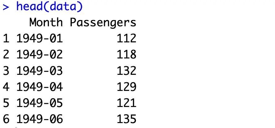
Next stop - feature engineering!

Date-Related Variables

The big difference when you first start using supervised learning algorithms for time series forecasting is that you have to construct a set of features. How detailed can you go depends on the data aggregation level. Our data is aggregated as monthly sums, which means we can extract columns such as season, month, and year.

The custom `get_season()` function calculates the season of the year, and is applied to the `Month` column of the dataset:

get_season <- function(mon) {
  if (mon %in% 3:5) {
    return("Spring")
  } else if (mon %in% 6:8) {
    return("Summer")
  } else if (mon %in% 9:11) {
    return("Autumn")
  } else {
    return("Winter")
  }
}

data <- data %>%
  mutate(Month = as.yearmon(Month)) %>%
  mutate(
    Year = year(Month),
    Month = month(Month),
    Season = sapply(Month, get_season)
  )

Onto the lag variables next.

Lag Variables

In the context of time series analysis, lag variables are values of a variable at previous time points. In other words, they represent past observations of the variables and are generally used to model the relationship between the value now and the value at previous times.

Think of it this way: The value of passengers in December 1955 will be somewhat connected to the value of passengers in November 1955 and months prior. For machine learning, you want to extract these features so the model can have a better chance of giving accurate results.

We’ll create 12 columns, representing lag variables of up to 12 periods. This means we’ll lose the information on the first 12 rows of the dataset since there’s no way to calculate their lagged values. That’s a tradeoff you have to live with, and to solve the issue of missing values, we’ll simply remove them:

lag_cols <- lapply(1:12, function(i) {
  lag(data$Passengers, i)
})
names(lag_cols) <- paste0("Lag", 1:12)
data <- cbind(data, lag_cols)
data <- na.omit(data)

data <- data %>%
  relocate(Year, .before = Month) %>%
  relocate(Passengers, .after = last_col())

head(data)

This is what the dataset looks like now:

As you can see, we have 15 features in total that will serve as predictors for the `Passengers` column. Up next, let’s split this dataset into training and testing portions.

Train/Test Split

The idea is to evaluate the model on the last 2 years of data and train it on everything else. In the Airline passengers dataset, the cutoff point where the test set starts in January of 1959:

test_set_start_year <- 1959
train_set <- subset(data, Year < test_set_start_year)
test_set <- subset(data, Year >= test_set_start_year)

dim(train_set)
dim(test_set)

Here’s what we’re working with:

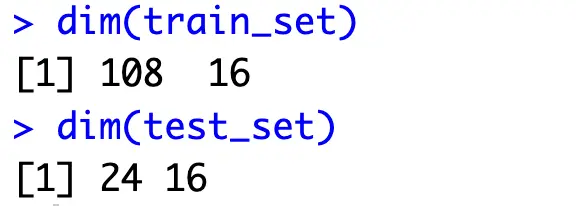
So, 9 years for training and 2 for evaluation. Not a whole lot, but maybe it’ll be enough.

Train and Evaluate Linear Regression Model on Time Series Data in R

This section will walk you through training a linear regression for a time series dataset. The procedure is quite straightforward, so let’s dive into it!

Training and Forecasting

The `lm()` function in R allows you to write a formula on which a linear regression model will be trained. We’re predicting `Passengers` and want to use all features available in `train_set`:

lm_model <- lm(Passengers ~ ., data = train_set)
summary(lm_model)

The model summary will tell us quite a bit about the model and the most relevant features:

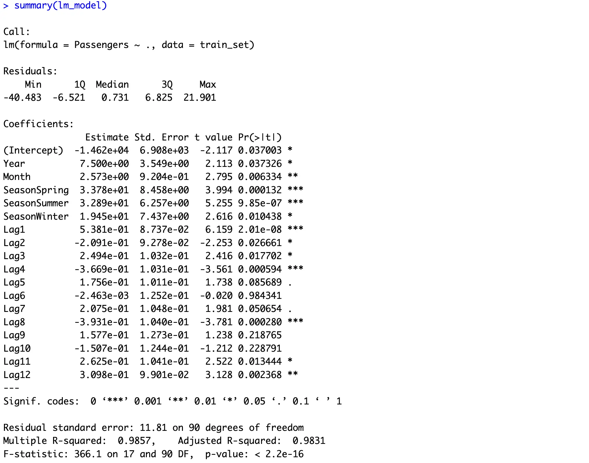
In a nutshell, almost all features are relevant for predictions (indicated by stars) and the model accounts for almost all the variance in the training set.

Now to calculate predictions, you can use the `predict()` function, pass in a model, and previously unseen data:

predictions <- predict(lm_model, newdata = test_set)
predictions

These are the results you’ll get:

Not much useful in this format, so let’s inspect the predictions graphically.

Forecast Visualization

Before creating a chart, we’ll construct three dataframes with identical column names and data formats. This will make it easier to visualize training data, testing data, and predictions:

viz_train_set <- data.frame(
  Period = as.yearmon(paste(train_set$Year, sprintf("%02d", train_set$Month), sep = "-")),
  Passengers = train_set$Passengers
)
viz_test_set <- data.frame(
  Period = as.yearmon(paste(test_set$Year, sprintf("%02d", test_set$Month), sep = "-")),
  Passengers = test_set$Passengers
)
viz_pred_set <- data.frame(
  Period = as.yearmon(paste(test_set$Year, sprintf("%02d", test_set$Month), sep = "-")),
  Passengers = predictions
)

Now using `ggplot2`, you can create a dedicated line for each dataset:

ggplot() +
  geom_line(data = viz_train_set, aes(x = Period, y = Passengers, color = "Training", group = 1), size = 1) +
  geom_line(data = viz_test_set, aes(x = Period, y = Passengers, color = "Testing", group = 1), size = 1) +
  geom_line(data = viz_pred_set, aes(x = Period, y = Passengers, color = "Predictions", group = 1), size = 1) +
  labs(
    title = "Airline Passengers - Predictions with Linear Regression",
    x = "Date",
    y = "Passengers"
  ) +
  scale_color_manual(values = c("Training" = "#12355B", "Testing" = "#D72638", "Predictions" = "#FFBA08"), name = "Airline passengers") +
  theme_minimal() +
  theme(plot.title = element_text(size = 20))

Here are the results:

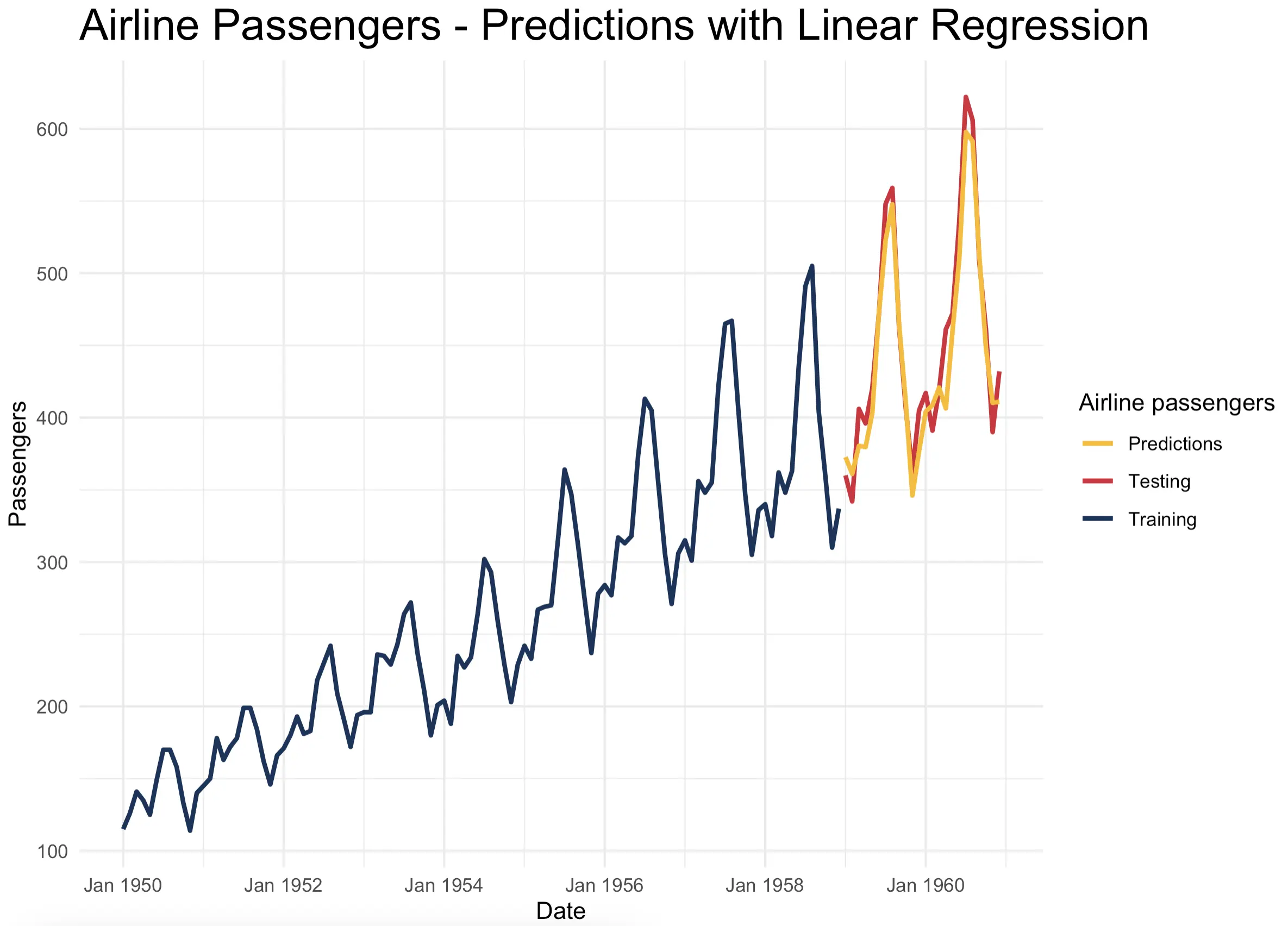
The predictions are almost spot on! Just from the looks, the model seems to be more accurate when compared to dedicated time series models.

But what will the numbers say? Let’s evaluate the model numerically next.

Forecast Evaluation

We discussed in the previous article that you’ll want to use time series specific metrics when evaluating predictive models. Mean Absolute Error (MAE), Root Mean Squared Error (RMSE), and Mean Absolute Percentage Error (MAPE) will all do the job perfectly:

print(paste("MAE: ", mae(viz_test_set$Passengers, viz_pred_set$Passengers)))
print(paste("RMSE: ", rmse(viz_test_set$Passengers, viz_pred_set$Passengers)))
print(paste("MAPE: ", mape(viz_test_set$Passengers, viz_pred_set$Passengers)))

You should expect to see relatively low error values:

In terms of an average error, the model is about 16.66K passengers wrong, or 20K if you want to penalize larger errors more. In percentages, that’s only about 3.7%. Just to recap, our best result with traditional time series algorithms was 6.7% for the percentage error. Huge improvement!

How to Predict Time Series Data Into the Unknown Future with Machine Learning Models

Forecasting time series data on a test set is easy - you already have everything you need. The complexity escalates quickly when you try to bring the forecasting logic into the unknown future, as you have to predict data points individually and calculate lag values based on predictions.

Let’s see what’s that all about.

Model Training

First things first, train the model on the entire dataset, not only the training set:

lm_model <- lm(Passengers ~ ., data = data)
summary(lm_model)

These are the summary statistics you’ll get:

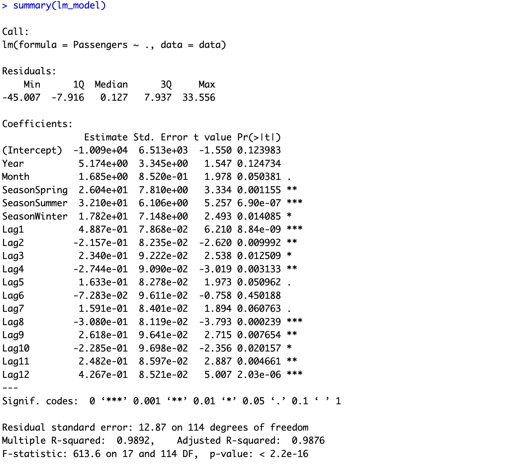
Once again, almost all features are relevant for the model’s predictive performance - nothing new to report.

Prediction Pipeline for the Unknown Future

Let’s discuss the prediction pipeline now. We’ll write a function `time_series_lm_predict()` that allows you to pass in the source data, model, and number of periods in the future you want to predict.

The function does the following:

• Constructs a prediction start year and month based on the maximum date value provided in `source_data`.
• Creates a data frame for the predictions by iterating up to `n_periods` and appending prediction year and month. In this step, the function also checks if the month is greater than 12, and if so, the year value is incremented.
• Extracts initial lags - reverse ordered last 12 values of the `source_data`. These will be updated on the fly.
• Iterates over all rows in `prediction_dates`, extracts the current row, constructs additional columns for lag variables, and makes a single-row prediction by using the provided `model`. Once done, the prediction is appended to the vector of predictions, and lags are updated so that the prediction is placed on the start, and the last lag value is removed.
• Returns a data frame of year-month combinations and predicted passenger values.

If you think that’s a lot, well, that’s because it is. But there’s no way around it. You must base predictions on previous predictions, as that’s the only way to predict the unknown future.

Here’s the full code snippet for the function:

time_series_lm_predict <- function(source_data, model, n_periods) {
  # To store the results
  predictions <- c()

  # Year and month to start predictions from
  start_year <- max(source_data$Year) + 1
  start_month <- 1
  # These wil be used in a loop
  yr <- start_year
  mt <- start_month
  # Empty dataframe to hold prediction dates
  prediction_dates <- data.frame()

  # Iterate to n_periods
  for (i in 1:n_periods) {
    # Add a row to the dataframe
    prediction_dates <- rbind(prediction_dates, data.frame(Year = yr, Month = mt))
    # Increment month
    mt <- mt + 1
    # Check if invalid month value, if so, reset it and increment year
    if (mt > 12) {
      mt <- 1
      yr <- yr + 1
    }
  }

  # Extract the last 12 passenger values in reverse order - these will serve as intial lag. values
  last_n_lags <- rev(source_data$Passengers[(length(source_data$Passengers) - 12 + 1):length(source_data$Passengers)])

  # Iterate over all prediction dates
  for (i in 1:nrow(prediction_dates)) {
    row <- prediction_dates[i, ]

    # Create a dataframe of lag values
    lag_data <- data.frame(matrix(last_n_lags, ncol = length(last_n_lags)))
    names(lag_data) <- paste0("Lag", 1:length(last_n_lags))

    # Create a single row for prediction
    prediction_data <- cbind(
      row,
      data.frame(
        Season = sapply(row$Month, get_season)
      ),
      lag_data
    )

    # Calculate prediction and convert it to integer
    prediction <- as.integer(predict(model, newdata = prediction_data))
    # Keep track of predictions
    predictions <- c(predictions, prediction)

    # Prepend to lags - prediction at time T is a first lag value for prediction at time T+1
    last_n_lags <- c(prediction, last_n_lags[-length(last_n_lags)])
  }

  return(data.frame(
    Year = prediction_dates$Year,
    Month = prediction_dates$Month,
    Passengers = predictions
  ))
}

You can now use the function to make time series forecasts using a linear regression model, let’s say for 24 months:

lm_predictions <- time_series_lm_predict(source_data = data, model = lm_model, n_periods = 24)
lm_predictions

Here are the predicted values:

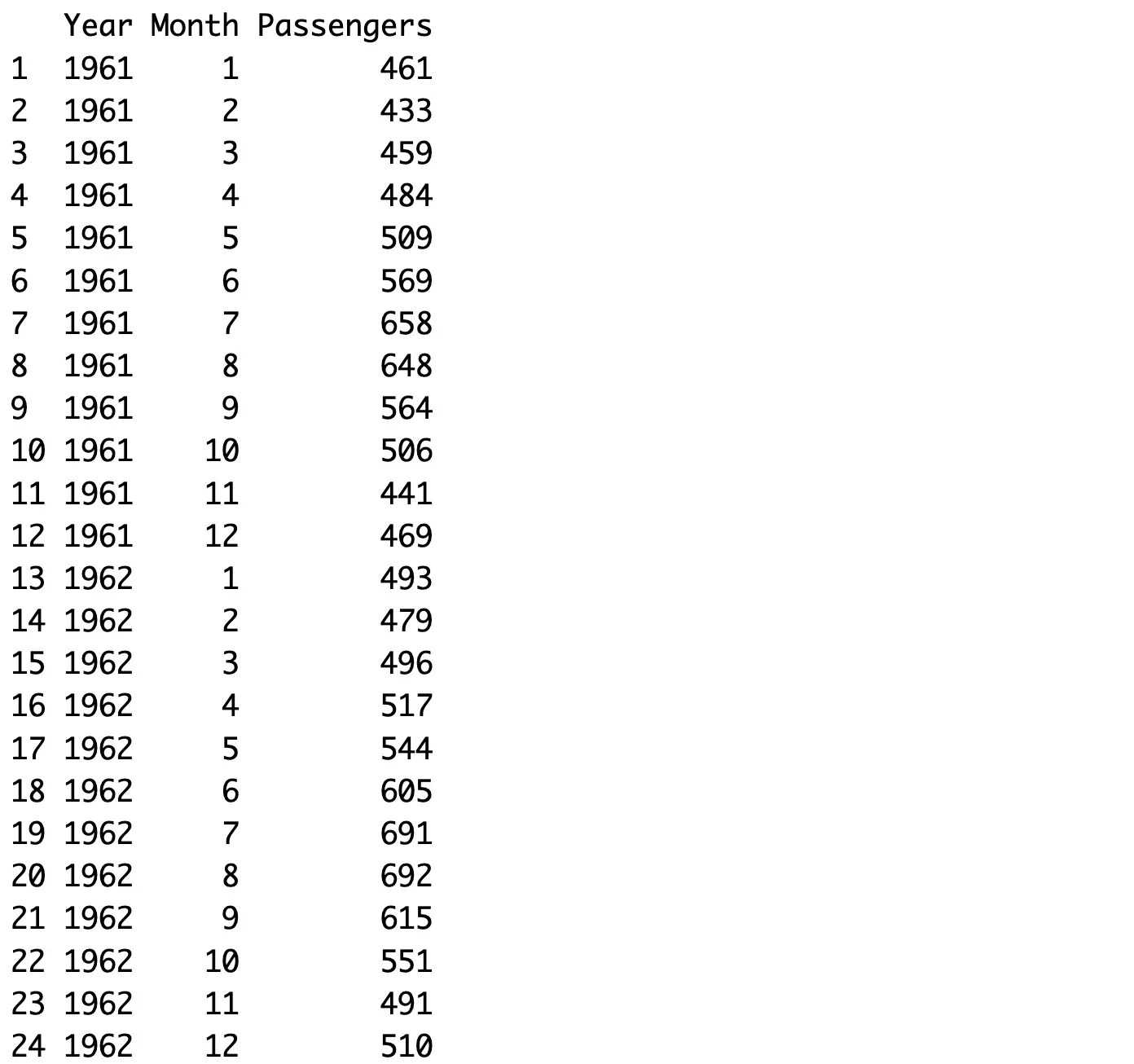
Our functions seem to work like a charm! Up next, let’s if predictions make sense.

Prediction Visualization

There’s no numerical way to evaluate our new set of predictions since there’s no data to compare it with. The only option you have is visualization.

Start by converting the full source dataset and predictions into a unified format:

viz_train_set <- data.frame(
  Period = as.yearmon(paste(data$Year, sprintf("%02d", data$Month), sep = "-")),
  Passengers = data$Passengers
)
viz_pred_set <- data.frame(
  Period = as.yearmon(paste(lm_predictions$Year, sprintf("%02d", lm_predictions$Month), sep = "-")),
  Passengers = lm_predictions$Passengers
)

And then, use the code snippet from earlier in the article to visualize both sets:

ggplot() +
  geom_line(data = viz_train_set, aes(x = Period, y = Passengers, color = "Training", group = 1), size = 1) +
  geom_line(data = viz_pred_set, aes(x = Period, y = Passengers, color = "Predictions", group = 1), size = 1) +
  labs(
    title = "Airline Passengers - Predictions with Linear Regression",
    x = "Date",
    y = "Passengers"
  ) +
  scale_color_manual(values = c("Training" = "#12355B", "Predictions" = "#FFBA08"), name = "Airline passengers") +
  theme_minimal() +
  theme(plot.title = element_text(size = 20))

The results speak for themselves:

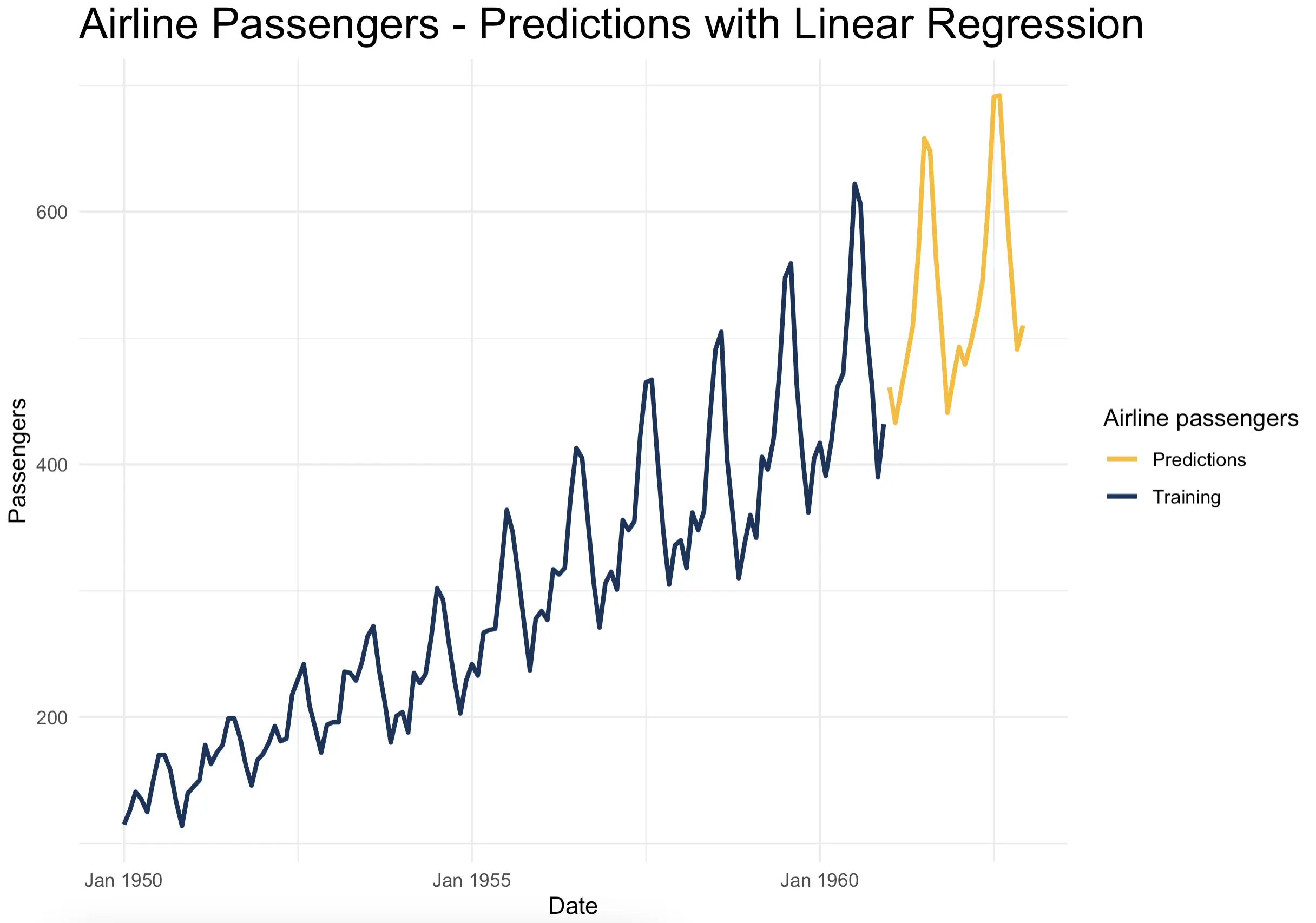
The predictions look like they belong. If the original data were to continue two years into the future, this is something you’ll likely see.

But the beauty of the `time_series_lm_predict()` function is that you can extend the forecasting period however far you want. You’ll get the following results if you set `n_periods = 60`, or 5 years into the future:

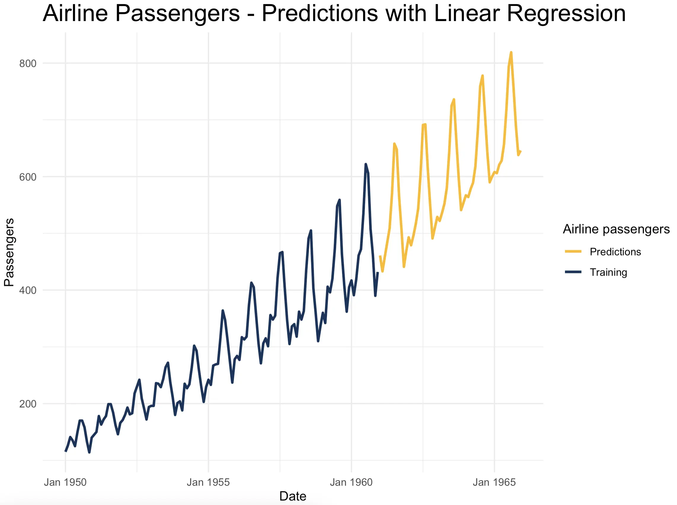
The trend and seasonality seem to match perfectly, but notice how the low periods get smoothed out. That’s the tradeoff of making predictions based on previous predictions. There’s not much you can do about it.

In the real world, it’s unlikely you’ll have to predict that much into the future with so few historical data points, so this smoothening side effect shouldn’t worry you too much.

Summing up Time Series Forecasting in R

To conclude, supervised machine learning algorithms are a viable option if you want to forecast time series data in R. The best part? We’ve only scratched the surface! There are so many machine learning algorithms to choose from and hyperparameters to tune. But that’s a topic for another time.

By now, you know the most important bit - methodology. You know how to go from a time series dataset to one applicable for supervised learning, and how to use the trained model to predict the future.

Take your time series charts to the next level by making them interactive and animated - All made possible with R Highcharts.