Most people are hesitant to learn new technologies unless they absolutely have to.

Data professionals are no exception. If you’ve learned SQL first, you’ll find a way to use it everywhere. Even if that means not learning about the benefits programming languages such as R and Python have to offer. You’re fine with that sacrifice. Until you aren’t.

R sqldf is a package that aims to bridge the gap for R newcomers with a decent SQL background. In plain English, you can play with R dataframes by writing SQL. No dplyr (or an equivalent). No hundreds of new methods you need to learn and relearn.

‍Eager to get started? So are we.

Need to process millions of rows in seconds? Try DuckDB, now with native R support.

Table of contents:

• R sqldf: An Introduction
• Hands-on R sqldf vs. dplyr - Which Package is Better for Beginners?
• Summing Up R sqldf

R sqldf: An Introduction

The sqldf package allows you to run SQL queries directly on R dataframes.

It can be a godsend for those more comfortable with SQL or situations where SQL feels more natural and straightforward. There’s a lot of “magic” happening behind the scenes, but for now, just remember that you can manipulate R dataframes as if they were tables in a database.

R sqldf uses SQLite as the backend for SQL queries, but you can configure it to use other databases if needed. This extensive FAQ section shows examples for H2 and PostgreSQL. TL;DR - it boils down to installing an R package for the given database vendor (e.g., `RPostgreSQL`), establishing a database connection, and then changing the value for `sqldf.driver` in `options()`.

Out of the scope for today.

While sqldf is an amazing tool for those with SQL background, we still recommend learning R’s suite of packages for data manipulation and analysis. Not just because we like R, but because of the fact sqldf isn’t as performant, especially on large datasets. R dplyr and dtplyr are your friends.

If you still want to take sqldf for a spin, install it with the following command:

install.packages("sqldf")

Then in a new R script, copy the following:

library(dplyr)
library(sqldf)
data("iris")

That’s all you need to follow along. Let’s go over some examples next.

Hands-on R sqldf vs. dplyr - Which Package is Better for Beginners?

We’ll show the differences between dplyr and sqldf in this section. By the end, you’ll have a clear idea of how much work it would require to fully migrate from SQL to R.

Simple Select

Let’s start simple and see what it takes to show the first 10 rows. With dplyr, you can use the `slice_head()` function, and with SQL, `LIMIT` is the keyword you’re looking for:

res_r <- iris %>%
  slice_head(n = 10)

res_sqldf <- sqldf("
  SELECT *
  FROM iris
  LIMIT 10
")

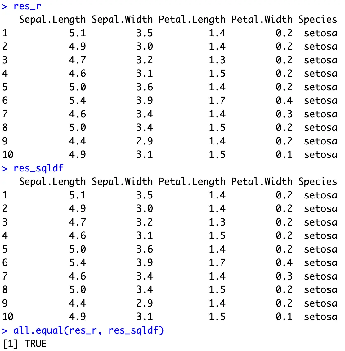
In R, you can also call `head(iris)` to do the same, but we’re sticking with dplyr for all of the examples.

Data Filtering

One of the first things you’ll learn in any data analysis course is all the different ways you can narrow down the results.

In R dplyr, that’s done with the `filter()` function, and in SQL, you’ll want to use the `WHERE` clause. In R, multiple filtering operations are separated by a comma, while in SQL, they’re separated with `AND`.

The Iris dataset has the misfortune of having dots in column names. The sqldf package doesn’t like that, since dot is used for different things.

Use `[]` to get around that:

res_r <- iris %>%
  filter(Petal.Length > 6)

res_sqldf <- sqldf("
  SELECT *
  FROM iris
  WHERE [Petal.Length] > 6
")

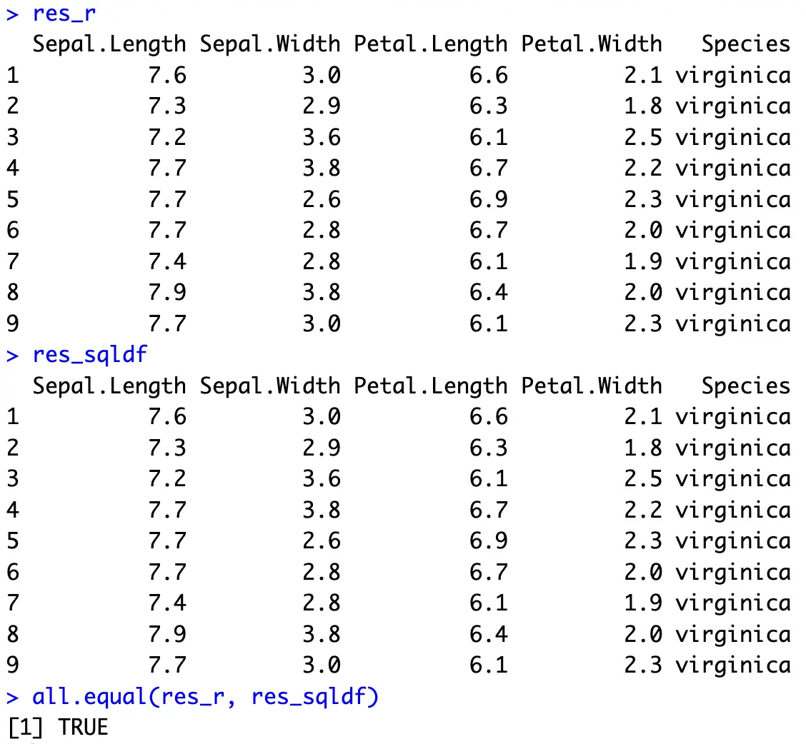
Both result sets are identical and show only the records in which the `Petal.Length` attribute is greater than 6.

Data Sorting

Another typical data operation is sorting the dataset by one or more columns, either in ascending or descending order.

In R dplyr, this is achieved through the `arrange()` function that sorts in ascending order by default. You can change that behavior by surrounding the column name with `desc()`. Multiple sorting conditions are separated by a comma.

On the other hand, SQL uses the `ORDER BY` clause. It also sorts in ascending order by order by default, and to change it, write `DESC` after the column name:

res_r <- iris %>%
  arrange(
    desc(Sepal.Width),
    Petal.Length
  ) %>%
  slice_head(n = 10)

res_sqldf <- sqldf("
  SELECT *
  FROM iris
  ORDER BY [Sepal.Width] DESC,
           [Petal.Length]
  LIMIT 10
")

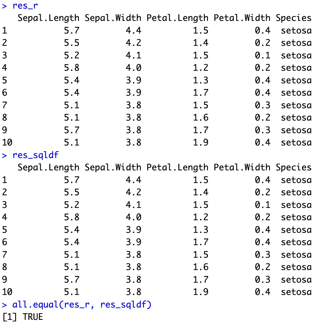
Both result sets show the first 10 entries sorted descendingly by `Sepal.Width` first, and then ascendingly by `Petal.Length`.

Aggregate Functions

More often than not, you’ll be tasked to get some summary statistics from the data.

This typically involves grouping the dataset by some categorical variable first, and then calculating the summary statistic for each group. Without grouping, you’ll end up with a summary statistic for an entire dataset.

In R, you first want to use the `group_by()` function to group the data by a provided column, and then call `summarise()` to create new summary statistics columns for each group. The `as.data.frame()` call at the end is optional, and is here just to ensure both result sets are in identical formats.

In SQL, you’ll want to call an aggregate function, such as `AVG()` on a column or columns of your choice, and then stick a `GROUP BY` expression at the end of the SQL snippet, but above any ordering operation:

res_r <- iris %>%
  group_by(Species) %>%
  summarise(avg_sepal_length = mean(Sepal.Length)) %>%
  as.data.frame()

res_sqldf <- sqldf("
  SELECT
    Species,
    AVG([Sepal.Length]) AS avg_sepal_length
  FROM iris
  GROUP BY Species
")

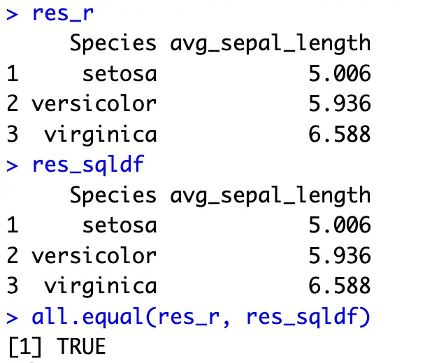
The above operation shows an average `Sepal.Length` value between the `Species` available in the dataset.

Unions

Unions are used to combine the results of two SQL queries or two R dataframe objects. `UNION ALL` keeps eventual duplicates, while `UNION` removes them.

The R example shows how to use the `bind_rows()` function to combine two R data frames, essentially performing an `UNION ALL` operation. The two subsets are firstly created, just to get the idea of having data stored in two separate objects.

On the other hand, everything is done in one SQL statement with sqldf. The `UNION ALL` keyword combines two result sets:

subset_1 <- iris %>%
  filter(
    Species == "setosa",
    Petal.Length > 1.5
  )
subset_2 <- iris %>%
  filter(
    Species == "versicolor",
    Petal.Length > 5
  )
res_r <- bind_rows(subset_1, subset_2)

res_sqldf <- sqldf("
  SELECT *
  FROM iris
  WHERE Species = 'setosa'
  AND   [Petal.Length] > 1.5
  UNION ALL
  SELECT *
  FROM iris
  WHERE Species = 'versicolor'
  AND   [Petal.Length] > 5
")

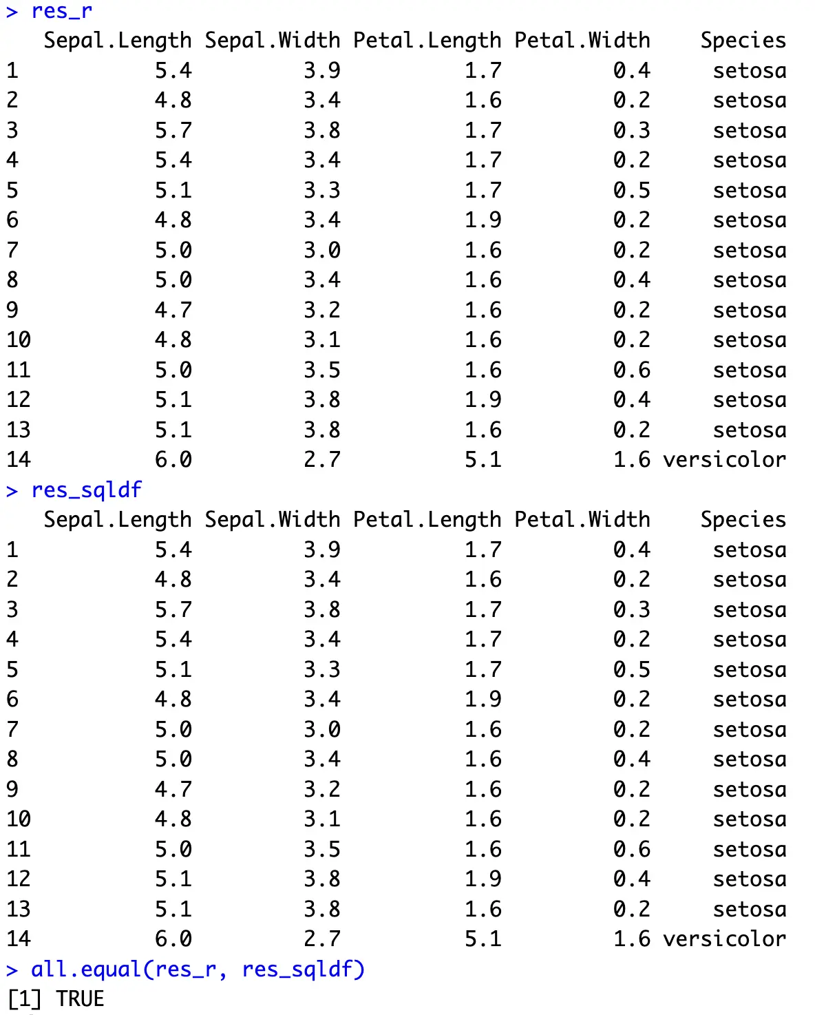
In the end, you’re basically stacking two data subsets vertically.

Joins

Most well-designed database systems store data in normalized tables, meaning the data isn’t redundant. For analytics, you often want to show an attribute measured through various columns, coming from 2 or more tables (denormalized results).

That’s where joins come in.

To demonstrate, let’s first add an ID column to the Iris dataset, and create a new subset with two additional columns - `Plant_Height` and `Soil_Type`:

iris_with_id <- iris
iris_with_id$ID <- 1:nrow(iris_with_id)

iris_subset <- data.frame(
  ID = c(1, 5, 10, 50, 100),
  Plant_Height = c(10.5, 15.2, 9.8, 14.7, 12.3),
  Soil_Type = c("Loam", "Clay", "Sand", "Loam", "Clay")
)

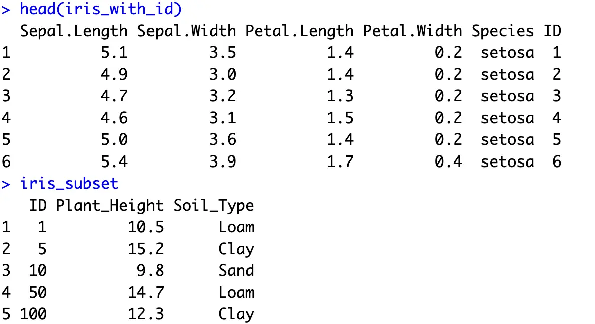
And now to combine the result sets horizontally, you can use an inner join. This will return only those rows that have a matching value for a given attribute in both sets. We’ll match the records through the `ID` attribute.

In R, this is done with the `inner_join()` function. You need to pass in the other dataframe object and the column you want to use for matching.

In SQL, joining is usually done by listing all the columns from different tables (and giving aliases to table names), and then using the `INNER JOIN` keyword to combine two tables on a given attribute:

res_r <- iris_with_id %>%
  inner_join(iris_subset, by = "ID")

res_sqldf <- sqldf("
  SELECT
    i.*,
    s.Plant_Height,
    s.Soil_Type
  FROM iris_with_id i
  INNER JOIN iris_subset s
    ON i.ID = s.ID
")

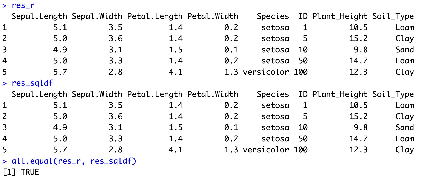
You now have more details on these 5 flowers. Other types of join would result in many missing values, especially `LEFT` and `OUTER`, assuming you have the original Iris dataset on the left part of the join.

Window Functions

And finally, let’s take a look at window/analytical functions.

These are your everyday aggregate functions followed by `OVER` and `PARTITION BY` keywords. You’ll usually want to use the window function when you need to perform calculations across a set of table rows that are somehow related to the current row.

To demonstrate, we’ll calculate the average `Sepal.Width` within each species and then calculate the difference between each observation’s `Sepal.Width` and the average of its species.

In R, this boils down to grouping the data by the target variable, calculating new columns, and ungrouping the results. For the sake of convenience, only the top 10 records are kept.

In SQL, all operations are done in the `SELECT` portion by using the earlier described keywords:

res_r <- iris %>%
  group_by(Species) %>%
  mutate(
    avg_sepal_width = mean(Sepal.Width),
    diff_from_avg = Sepal.Width - avg_sepal_width
  ) %>%
  ungroup() %>%
  slice_head(n = 10) %>%
  as.data.frame()

res_sqldf <- sqldf("
  SELECT
    [Sepal.Length],
    [Sepal.Width],
    [Petal.Length],
    [Petal.Width],
    Species,
    AVG([Sepal.Width]) OVER (PARTITION BY Species) AS avg_sepal_width,
    [Sepal.Width] - AVG([Sepal.Width]) OVER (PARTITION BY Species) AS diff_from_avg
  FROM iris
  LIMIT 10
")

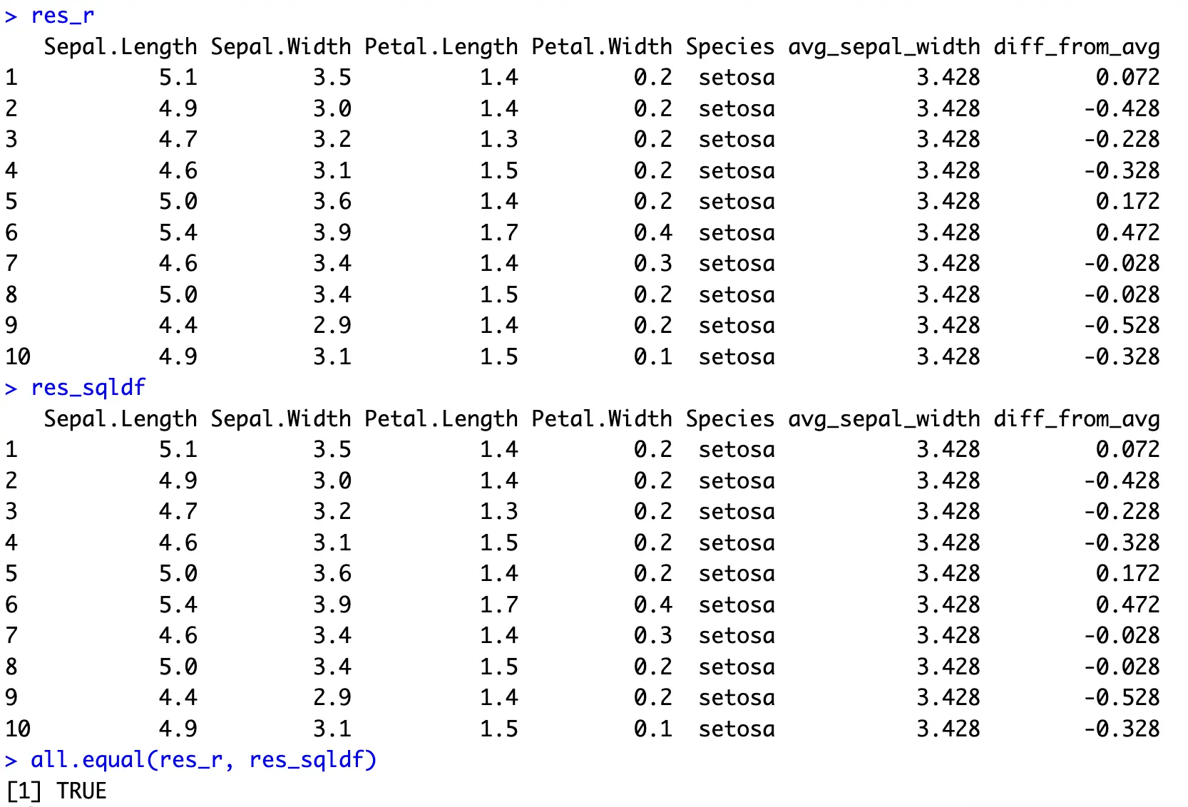
Not the most interesting example, but perfectly demonstrates what’s needed to bring SQL’s window function to R and dplyr.

Summing Up R sqldf

To conclude, R is super friendly to newcomers, assuming you possess the basic knowledge for working with data. Everyone knows SQL, and many data enthusiasts and professionals learn it before R. Packages like R sqldf make the transition that much easier.

Overall, it’s a great tool that can help you learn R-specific packages such as dplyr. Beyond that, especially for large dataset, we wouldn’t recommend it.

‍What are your thoughts on R sqldf? Are you using this package daily or have you considered it only to be a transition from SQL to R? Join our Slack community and let us know.

Which function implementation is faster? Don’t guess, use R Microbenchmark and be certain.