R Sidebot: How to Add an LLM Assistant to Your R Shiny Apps

Reading time:
time
min
By:
Dario Radečić
December 6, 2024

Imagine a dashboard where queries and filters are applied through natural text - that’s exactly what you’ll build today!

You already know that you can build R Shiny Applications with Generative AI, but this one is quite different. The goal is not to help you generate the source code but rather to allow the end user to ask questions, and have your dashboard elements updated automatically with relevant data.

In other words, Generative AI replaces traditional dropdown menus, sliders, input fields, and other data-filtering operations. It understands the semantics of your data and can successfully manipulate it based on user input (natural language). Even better, you can use it to explain charts to remove every level of uncertainty.

After reading this article, you’ll know how to use the R Sidebot project to add Generative AI functionality to your project. We'll show you how to run the original app, and how to customize it for your dataset.

Let’s dig in!

New to Machine Learning in R? Try tidymodels, a tidyverse-like ecosystem for machine learning in R.

Table of contents:

Why You Should (and Shouldn’t) Add an LLM to Your Shiny App

Adding an LLM to your app brings the user experience to a whole other dimension, but it’s not without its downsides. Before diving into the code, let’s first discuss some more generic pros and cons of using LLMs in your apps.

Pros of using LLMs

In terms of replacing traditional filters with an LLM in your application, there are some obvious benefits for the end user, so we’ll list a couple of them here:

  • Enhanced User Experience: Apps take time to learn, even those with a superb user experience. If users can quickly ask questions in natural language, their learning curve reduces drastically when compared to navigating through numerous filters and settings. Built-in chatbots provide intuitive and interactive responses which often results in a more engaging user session.
  • Easier Data Exploration: Your app or dashboard might contain some gold nuggets, but it doesn’t make a difference if the end user can’t get to them. Going through multiple filters is less user-friendly than asking a simple question like “Show me last month’s sales in Toronto” or something similar. It’s a critical win for everyone, especially for non-technical users.
  • Personalized Insights: You can configure the app in such a way that user preferences matter when it comes to response formatting. For example, some might prefer to-the-point changes in data and visuals, while others might prefer all of that plus natural language explanations.
  • Makes Complex Workflows Simpler: Imagine looking at your dashboard and wondering how many steps it will take to compare sales from this quarter to the previous quarter. It’s probably not something you can do in one click. With a chatbot, users can automate multi-step analyses and retrieve complex data with simple natural language commands.
  • Reduces Training and Support Costs: Because chatbots are intuitive, they minimize the learning curve for new users and hence decrease (or even eliminate) the need for extensive training.

Cons of using LLMs

It’s not all sunshine and rainbows, and you also have to be aware of potential drawbacks when replacing traditional web application filters with LLMs. These are:

  • Data Sharing: Your data, or at least your data scheme is shared with a third party (such as OpenAI). It might not be relevant to you for a personal pet project, but it’s almost never a good idea for enterprise projects dealing with sensitive data. You could mitigate this by self-hosting an LLM, but that comes with its own set of headaches.
  • Cost: Text embedding and running communicating with LLMs isn’t free, and it definitely won’t be cheap if you have a large user base. Like in the previous item, self-hosting an embedding and chat model might be a good idea here.
  • Answer Quality: LLMs are known to hallucinate, and getting around that is easier said than done. If you want every generated answer to be spot on, prepare to spend some time with prompt engineering.
  • Fallback Implementation: What happens if the chatbot can’t get the data query right? Or you run out of credits? Or if internet connection fails? There are many points of failure, so it’s wise to think ahead. Maybe give your user an option to switch between a chatbot and more traditional data filtering options on the application settings page.

You now know the positive and negative sides of using LLMs in your application for data manipulation purposes. Up next, you’ll get your hands dirty with R Sidebot.

R Sidebot: How to Get Started

The R Sidebot project is available on GitHub and requires minimal intervention to get it up and running on your machine. In this section, you’ll see how it works on the default tips application, and then in the later section, you’ll see how to modify it to work on your data.

Download the GitHub repo

To start, download the source code from the official GitHub repository:
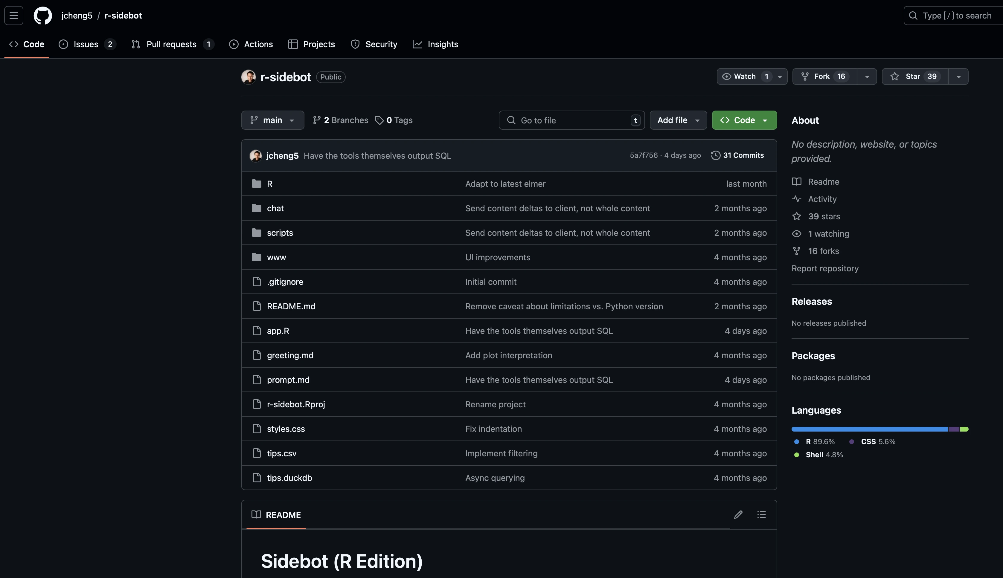
Image 1 - R Sidebot GitHub repo

The project contains application logic and data that shows you the Sidebot in action on the tips dataset.

To get started, you should run the following command from the R console (to install dependencies):

install.packages("pak")

pak::pak(c("bslib", "DBI", "dplyr", "duckdb", "fastmap", "fontawesome",
  "ggplot2", "ggridges", "here", "plotly", "reactable", "shiny",
  "hadley/elmer", "jcheng5/shinychat"))

That takes care of external R dependencies, however, the project is missing the OpenAI API key setup process, so let’s cover that next.

Setup OpenAI API key

Assuming you have an OpenAI account, head over to the API keys section in the Settings menu. Here, you’ll want to create a new API key (or reuse the one you already have):
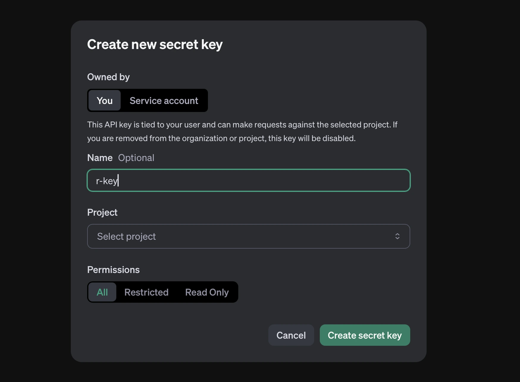
Image 2 - OpenAI API key generation (1)

The API key is now created, so make sure to copy its value somewhere safe - you won’t be able to see it from the OpenAI settings page in the future:
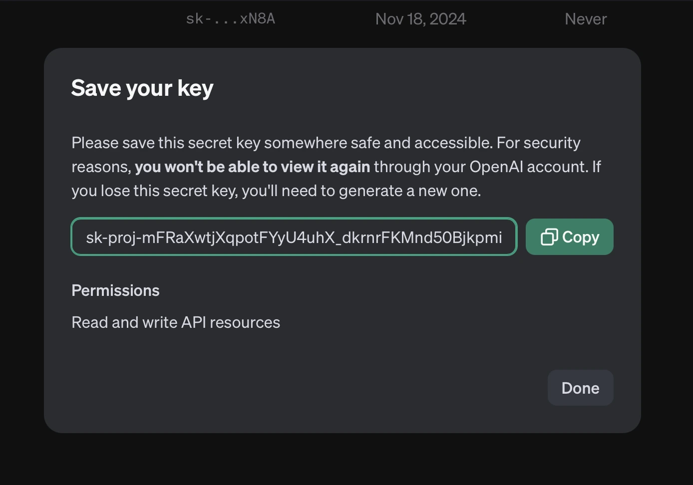
Image 3 - OpenAI API key generation (2)

Now, assuming you’ve already opened the downloaded Sidebot project in RStudio or Positron, create an `.Renviron` file and declare an environment variable named `OPENAI_API_KEY`. Paste your key after it, separated by the `=` sign:

Image 4 - Renviron file

You could set the environment variable in some different manner, but `.Renviron` file is among the most practical options. Just don’t forget to add it to `.gitignore`.

OpenAI quota error - How to fix it

You can now start the Shiny application, and the default data and charts will be rendered correctly:
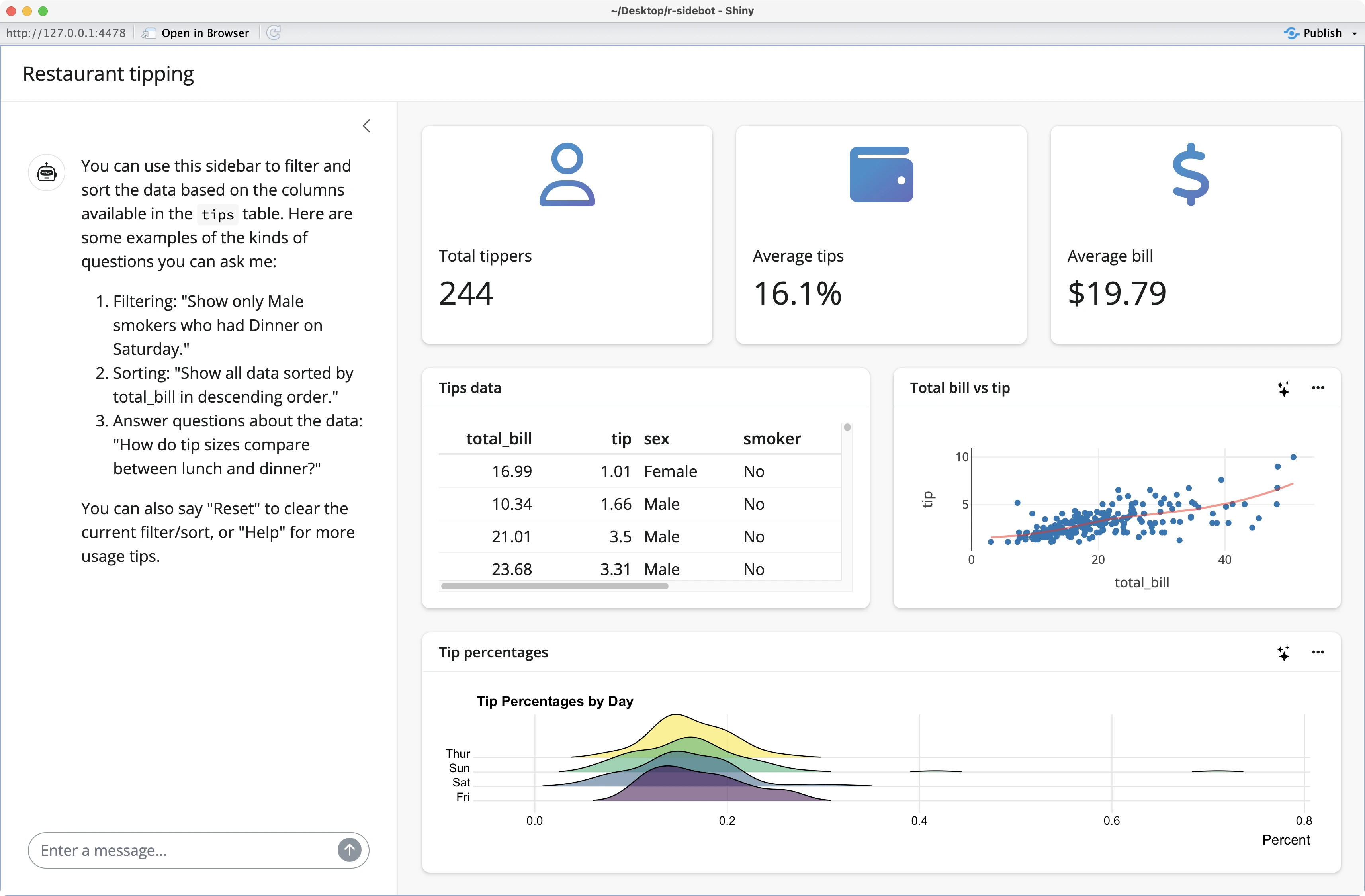
Image 5 - Sidebot demo app

You can even start asking questions in the sidebar, as you can see from our example below:
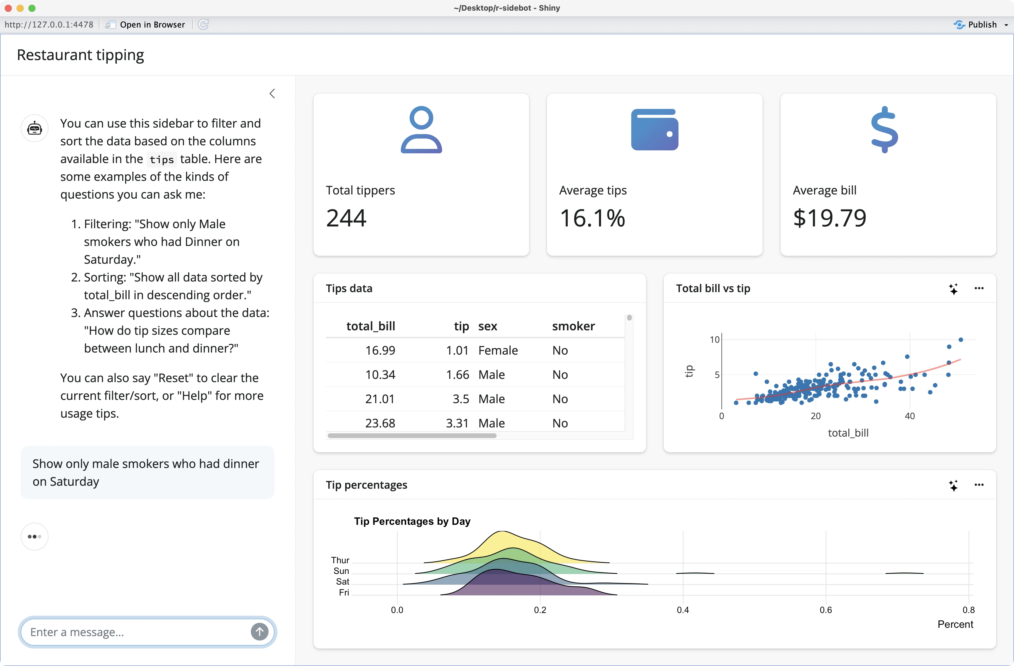
Image 6 - Sidebot demo app - asking questions

However, if you’re on a fresh OpenAI account, you’ll likely run into the `HTTP 429 Too Many Requests` error. It happens because your account has no credits:
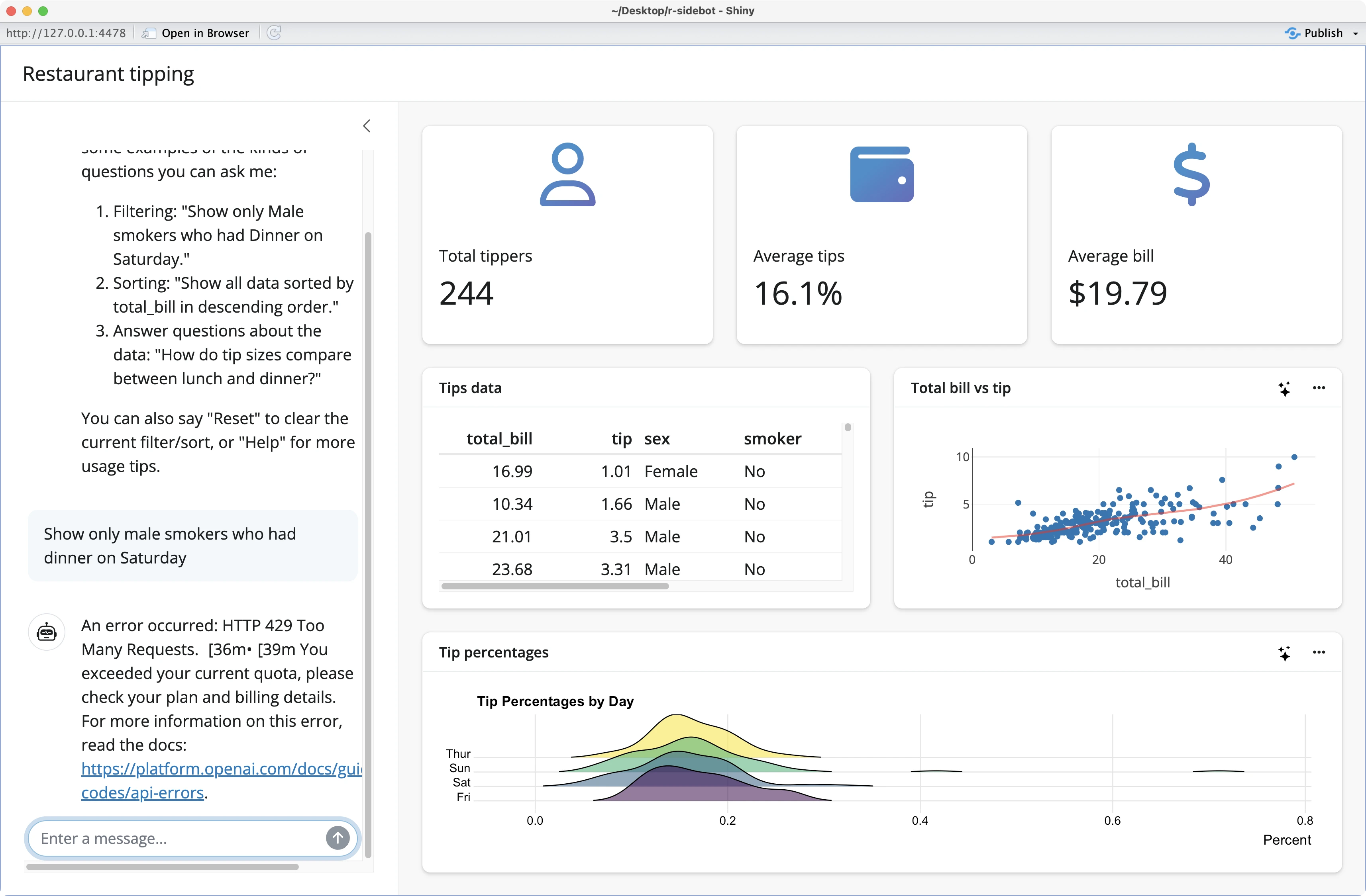
Image 7 - Sidebot demo app - quota error

To fix this, you have to go back to the OpenAI Settings page, add a Billing method, and add funds to your account. The minimum amount as of November 2024 is USD 5 (before taxes).

Once that’s out of the way, you’ll see available credits in your account:
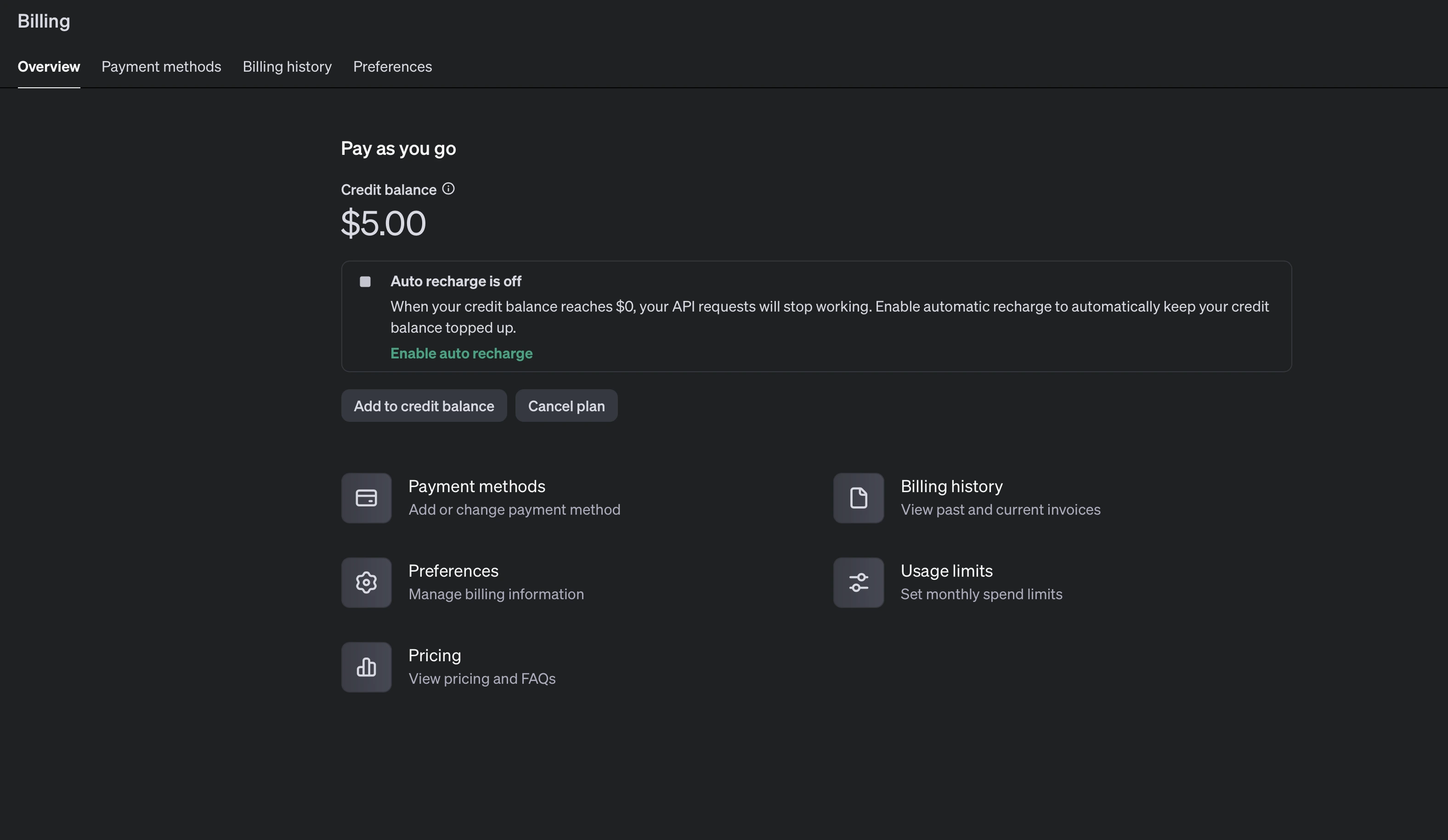
Image 8 - OpenAI balance

Hopefully, this should fix the `HTTP 429` error.

Response streaming error - How to fix it

If you restart your app, you’ll see another error message after submitting your question:
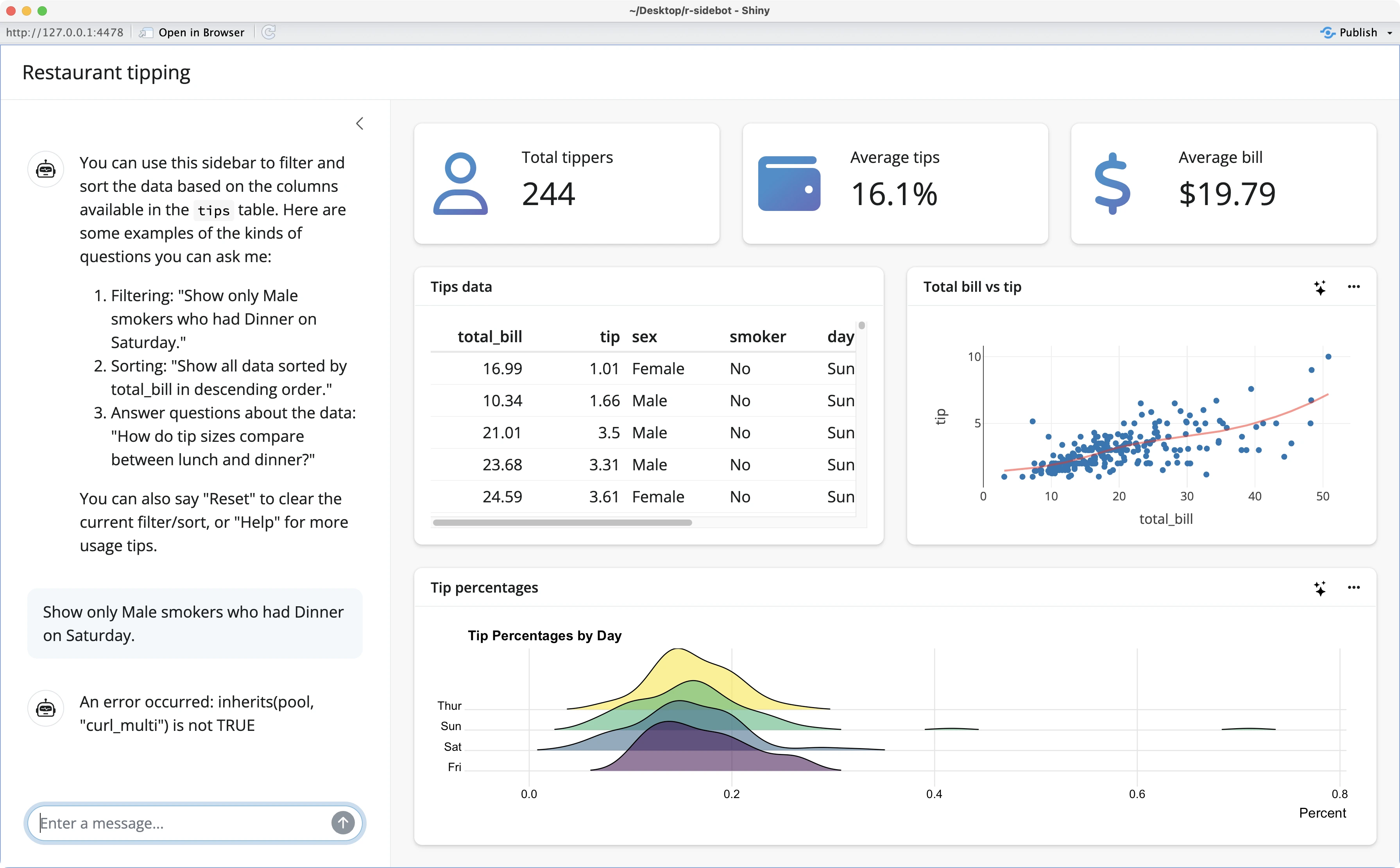
Image 9 - Chat streaming error

This one is a bit trickier to solve, but it boils down to Sidebot using a buggy `stream_async()` method to get the response back to the user. In `app.R` on line 355, swap it for the `chat_async()` method instead:

...
# Handle user input
  observeEvent(input$chat_user_input, {
    # Add user message to the chat history
    chat_append("chat", chat$chat_async(input$chat_user_input)) %...>% {
       # print(chat)
    }
  })
...

This is what your code should look like after the change:

Image 10 - Chat streaming error fix in app.R

And now finally, you’ll see the app updated after submitting your query through the chat interface:
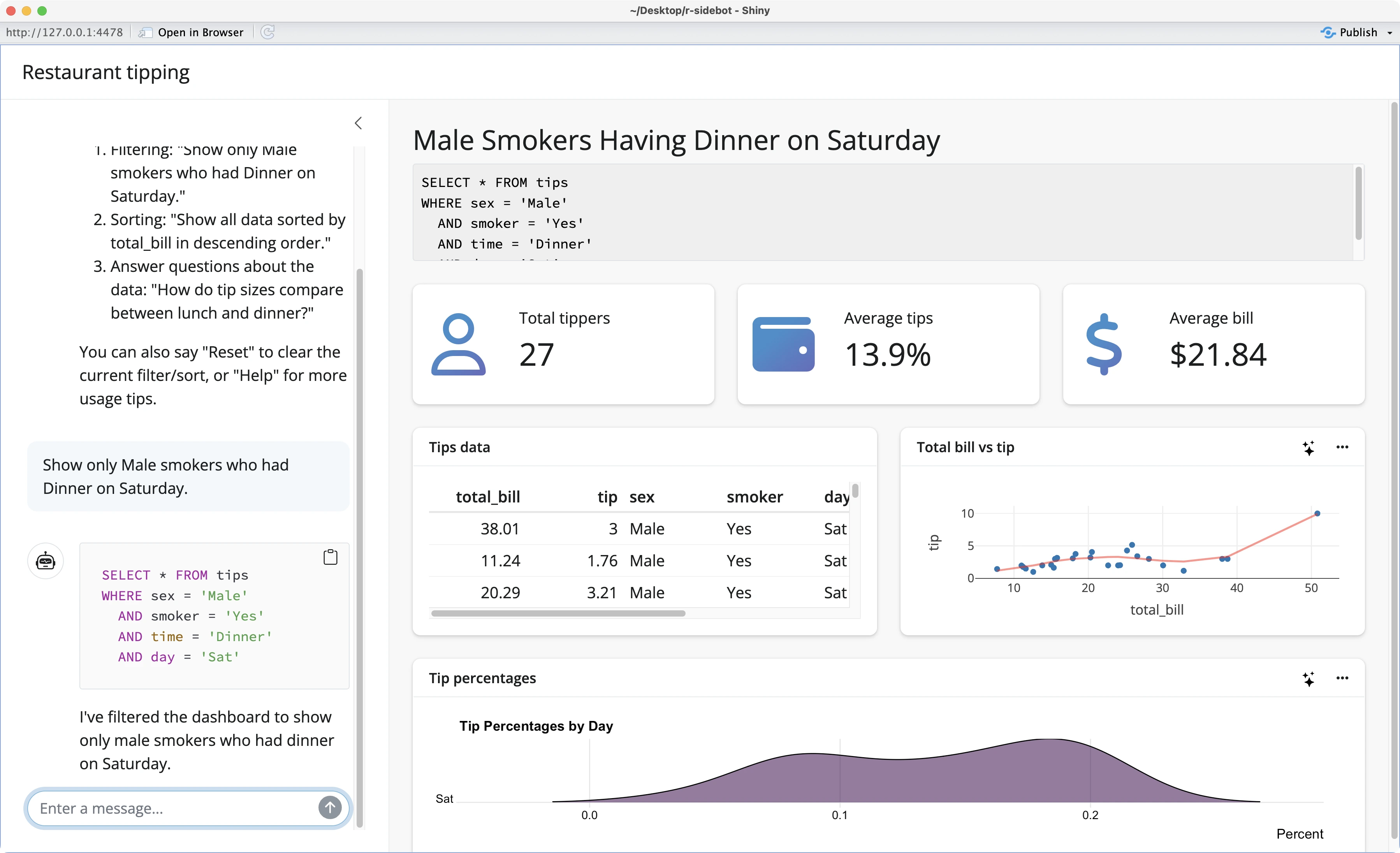
Image 11 - Application after filtering by LLM

Both charts in the dashboard have a familiar stars icon often used to represent AI features. When you click on it, you should see AI insights about the current charts.

Unfortunately, this doesn’t happen, and a familiar error message is displayed instead:
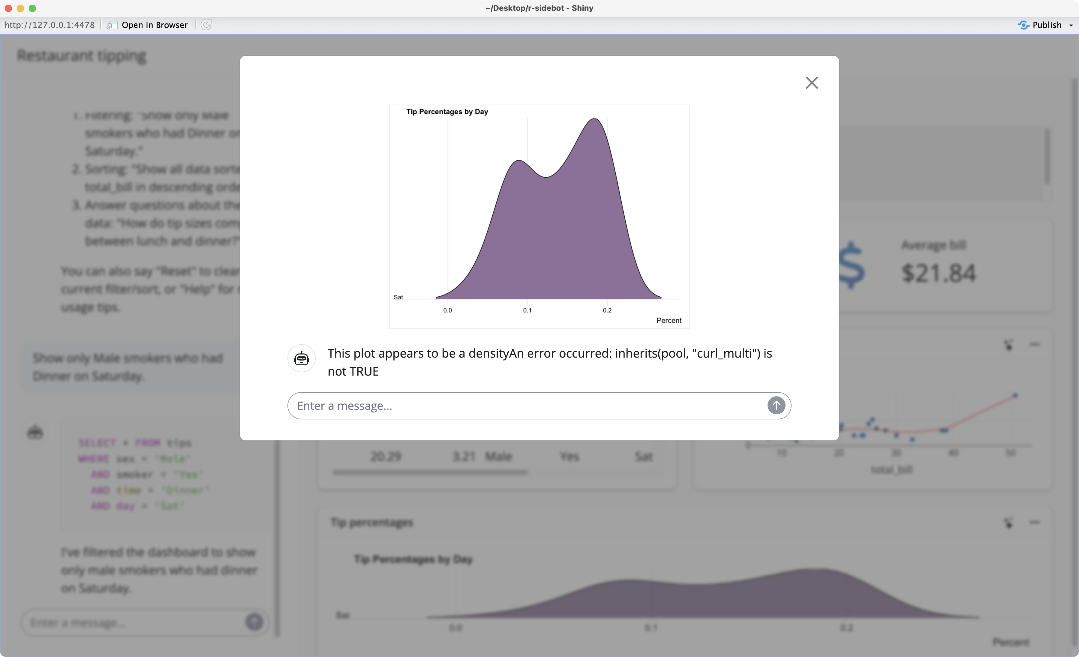
Image 12 - Chart explanation error

You already know how to fix it - replace `stream_async()` with `chat_async()` in two places in `R/explain-plot.R`:

...
session$onFlushed(function() {
    stream <- chat$chat_async(
      "Interpret this plot, which is based on the current state of the data (i.e. with filtering applied, if any). Try to make specific observations if you can, but be conservative in drawing firm conclusions and express uncertainty if you can't be confident.",
      img_content
    )
    chat_append(chat_id, stream)
  })

  observeEvent(session$input[[paste0(chat_id, "_user_input")]], {
    stream <- chat$chat_async(session$input[[paste0(chat_id, "_user_input")]])
    chat_append(chat_id, stream)
  })
...

This is what your code should look like after the change:

Image 13 - Chart explanation error fix in explain-plot.R

Restart the app once more, and you’ll be presented with a large text block of plot explanations:
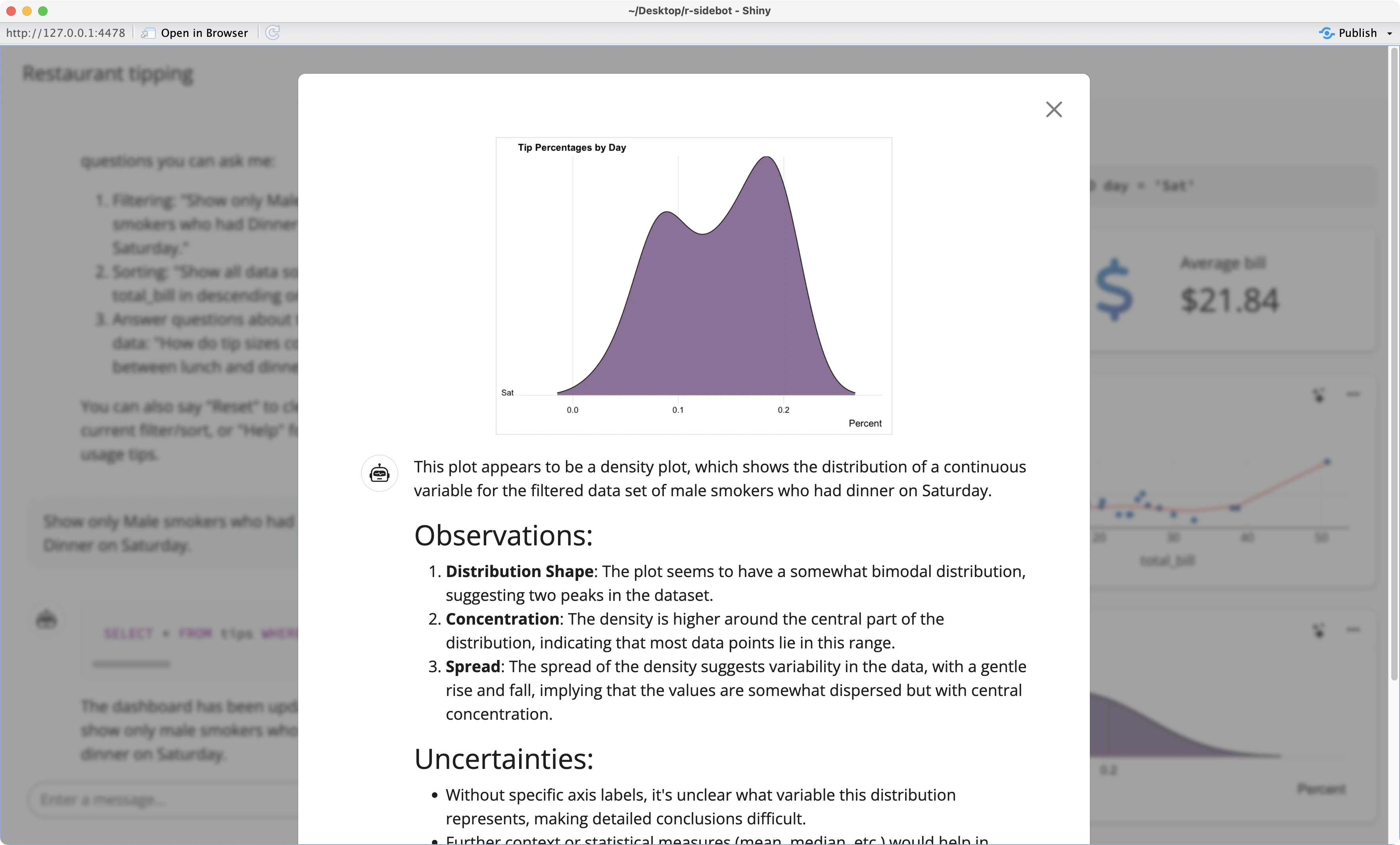
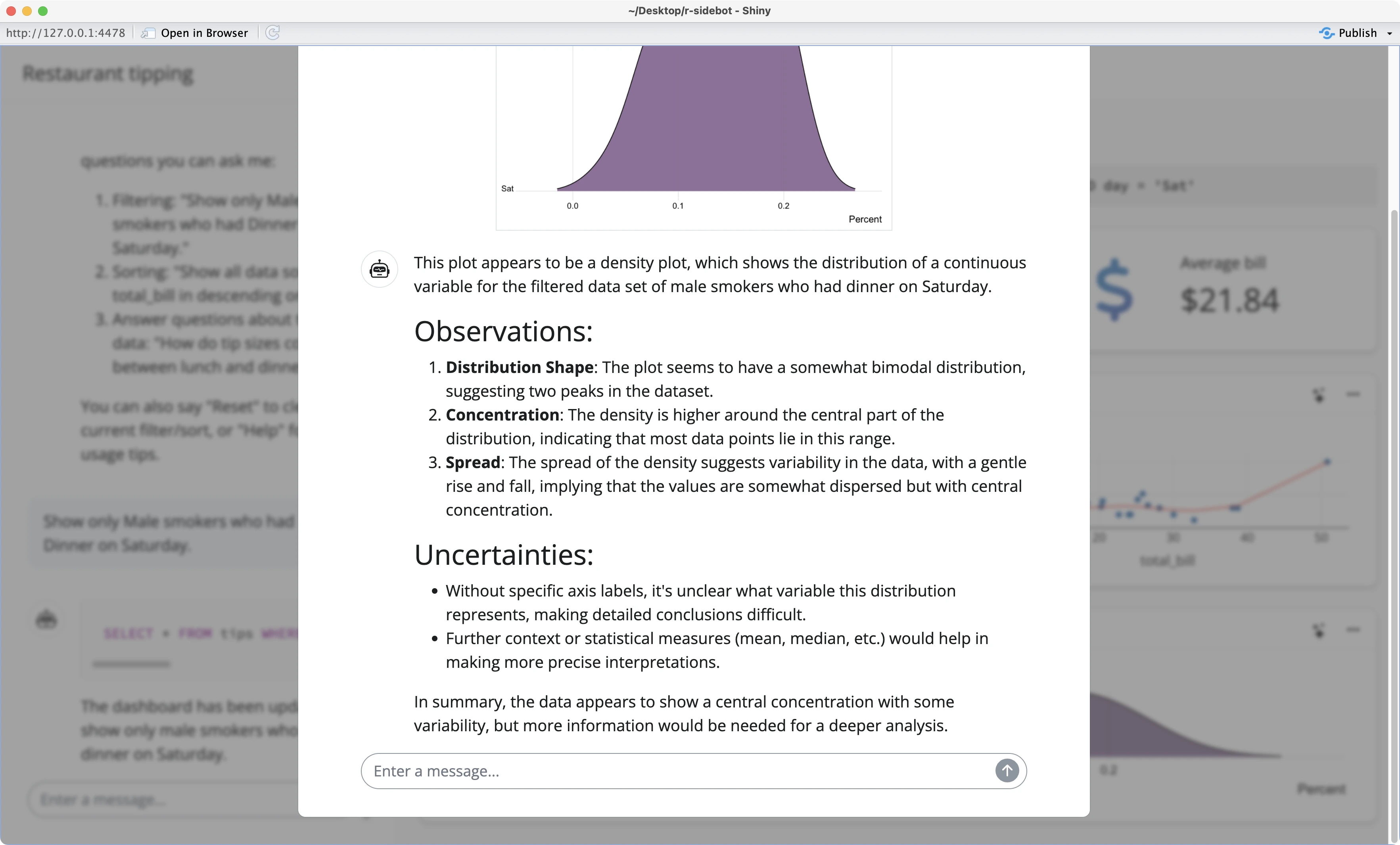
Image 14 - Chart explanation result (1)
Image 15 - Chart explanation result (2)

The R Sidebot app is now working as advertised on the tips dataset. Up next, you’ll see how to tweak the app so it works on other datasets as well.

R Sidebot: How to Customize the Assistant to Work on Your Data

In this section, you’ll see what it takes to customize R Sidebot to work on the Iris dataset.

Download the dataset

Start by downloading the dataset from a provided link. Store it as a CSV file in the project folder:
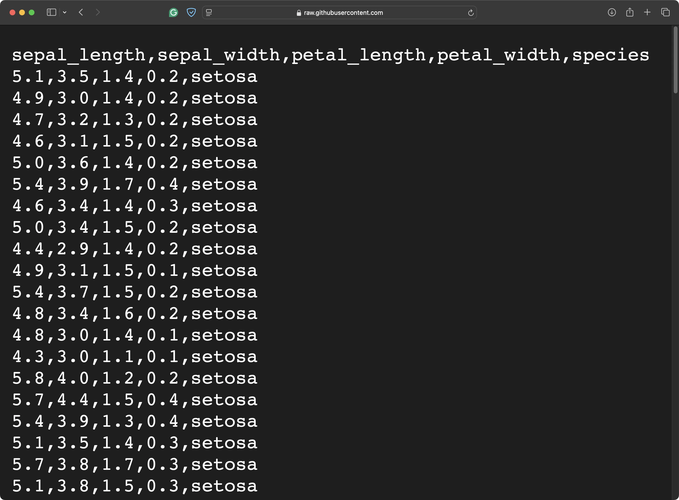
Image 16 - The Iris dataset

Convert CSV to DuckDB

Once downloaded, you’ll want to slightly tweak the `scripts/setup.R` file and run it so that the CSV file is converted to DuckDB. This is required so the Sidebot can generate SQL queries:

# scripts/setup.R

library(duckdb)
library(DBI)
library(here)

db_path <- here("iris.duckdb")

# Delete if exists
if (file.exists(db_path)) {
  unlink(db_path)
}

# Load tips.csv into a table named `tips`
conn <- dbConnect(duckdb(), dbdir = db_path)
duckdb_read_csv(conn, "iris", here("iris.csv"))
dbDisconnect(conn)

If you open the DuckDB file with a tool like TablePlus, you’ll see the dataset is stored in the `iris` table:
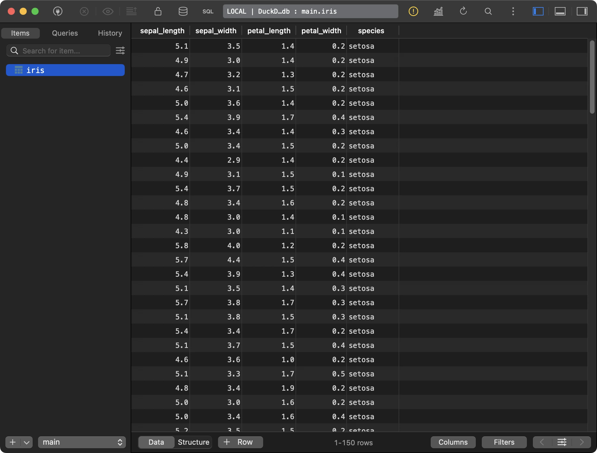
Image 17 - DuckDB table

Customize Markdown files

You might have noticed two markdown files in the project directory - `greeting.md` and `prompt.md`. We don’t want to overwrite them, so create two new files - `greetings_iris.md` and `prompt_iris.md`.

The latter is a direct copy, while the prior needs some modifications. In short, it represents the text shown to the user in the sidebar. Make sure to include helpful instructions on how to use the chatbot:

You can use this sidebar to filter and sort the data based on the columns available in the `iris` table. Here are some examples of the kinds of questions you can ask me:

1. Filtering: "Show me flowers of type setosa."
2. Sorting: "Sort the data by the sepal_length column in descending order."
3. Answer questions about the data: "What is the range of the petal_width column?"

You can also say "Reset" to clear the current filter/sort, or "Help" for more usage tips.

The `prompt.md` file serves as a system prompt, and you can just copy it to a new file.

Customize R scripts

Now inside `explain-plot.R`, you want to make sure you’re using the `chat_async()` method instead of `stream_async()`. If you’ve followed the previous section, no change is required here:

# scripts/explain-plot.R

library(ggplot2)

#' Convert a plot object to a PNG data URI
#'
#' @param p The plot object; currently, plotly and ggplot2 are supported. Note
#'     that plotly requires Python, {reticulate}, and the PyPI packages {plotly}
#'     and {kaleido}.
plot_to_img_content <- function(p) {
  UseMethod("plot_to_img_content", p)
}

plot_to_img_content.plotly <- function(p) {
  # Create a temporary file
  tmp <- tempfile(fileext = ".png")
  on.exit(unlink(tmp))

  # Save the plot as an image
  save_image(p, tmp, width = 800, height = 600)
  elmer::content_image_file(tmp, resize = "high")
}

plot_to_img_content.ggplot <- function(p) {
  # Create a temporary file
  tmp <- tempfile(fileext = ".png")
  on.exit(unlink(tmp))

  ggsave(tmp, p, width = 800, height = 600, units = "px", dpi = 100)
  elmer::content_image_file(tmp, resize = "high")
}

explain_plot <- function(chat, p, model, ..., .ctx = NULL, session = getDefaultReactiveDomain()) {
  chat_id <- paste0("explain_plot_", sample.int(1e9, 1))
  # chat <- chat$clone()

  img_content <- plot_to_img_content(p)
  img_url <- paste0("data:", img_content@type, ";base64,", img_content@data)

  showModal(modalDialog(
    tags$button(
      type="button",
      class="btn-close d-block ms-auto mb-3",
      `data-bs-dismiss`="modal",
      aria_label="Close",
    ),
    tags$img(
      src = img_url,
      style = "max-width: min(100%, 400px);",
      class = "d-block border mx-auto mb-3"
    ),
    chat_ui(chat_id),
    size = "l",
    easyClose = TRUE,
    title = NULL,
    footer = NULL,
  ) |> tagAppendAttributes(style = "--bs-modal-margin: 1.75rem;"))

  session$onFlushed(function() {
    stream <- chat$chat_async(
      "Interpret this plot, which is based on the current state of the data (i.e. with filtering applied, if any). Try to make specific observations if you can, but be conservative in drawing firm conclusions and express uncertainty if you can't be confident.",
      img_content
    )
    chat_append(chat_id, stream)
  })

  observeEvent(session$input[[paste0(chat_id, "_user_input")]], {
    stream <- chat$chat_async(session$input[[paste0(chat_id, "_user_input")]])
    chat_append(chat_id, stream)
  })
}

Customize app.R

And finally, let’s modify the `app.R` file. Here are the modifications we’ve made:

  • Load the `iris.duckdb` file.
  • Point to the newly created `greetings_iris.md` file for the sidebar contents.
  • Inside UI value boxes, tweak the top 3 cards to show a number of rows, average petal length, and average petal width. Output names are also updated, so this will have to be reflected in the server.
  • Remove the area plot.
  • Update the `server()` function to point to new data and update reactive data for the 3 tweaked UI components.
  • Remove area plot logic from the `server()` function.

It’s quite a bit of work, no arguing there. This is our final version of the `app.R` file:

library(shiny)
library(bslib)
library(promises)
library(fastmap)
library(duckdb)
library(DBI)
library(fontawesome)
library(reactable)
library(here)
library(plotly)
library(ggplot2)
library(ggridges)
library(dplyr)
library(elmer)
library(shinychat)


# Point to the newsly created DuckDB file
conn <- dbConnect(duckdb(), dbdir = here("iris.duckdb"), read_only = TRUE)
onStop(\() dbDisconnect(conn))
openai_model <- "gpt-4o"
# Change the system prompt since the table name is different now
system_prompt_str <- system_prompt(dbGetQuery(conn, "SELECT * FROM iris"), "iris")
# New markdown file
greeting <- paste(readLines(here("greetings_iris.md")), collapse = "\n")
icon_explain <- tags$img(src = "stars.svg")


ui <- page_sidebar(
  style = "background-color: rgb(248, 248, 248);",
  title = "Iris dataset",
  includeCSS(here("styles.css")),
  sidebar = sidebar(
    width = 400,
    style = "height: 100%;",
    chat_ui("chat", height = "100%", fill = TRUE)
  ),
  useBusyIndicators(),

  # 🏷️ Header
  textOutput("show_title", container = h3),
  verbatimTextOutput("show_query") |>
    tagAppendAttributes(style = "max-height: 100px; overflow: auto;"),

  # 🎯 Value boxes
  layout_columns(
    fill = FALSE,
    value_box(
      "Row count",
      textOutput("row_count", inline = TRUE)
    ),
    value_box(
      "Avg. petal length",
      textOutput("average_petal_length", inline = TRUE)
    ),
    value_box(
      "Avg. petal width",
      textOutput("average_petal_width", inline = TRUE)
    ),
  ),
  layout_columns(
    style = "min-height: 450px;",
    col_widths = c(6, 6, 12),

    # 🔍 Data table
    card(
      style = "height: 500px;",
      card_header("Iris data"),
      reactableOutput("table", height = "100%")
    ),

    # 📊 Scatter plot
    card(
      card_header(
        class = "d-flex justify-content-between align-items-center",
        "Petal length vs. Petal width",
        span(
          actionLink(
            "interpret_scatter",
            icon_explain,
            class = "me-3 text-decoration-none",
            aria_label = "Explain scatter plot"
          ),
          popover(
            title = "Add a color variable", placement = "top",
            fa_i("ellipsis"),
            radioButtons(
              "scatter_color",
              NULL,
              c("none", "sex", "smoker", "day", "time"),
              inline = TRUE
            )
          )
        )
      ),
      plotlyOutput("scatterplot")
    )
  )
)


server <- function(input, output, session) {
  # 🔄 Reactive state/computation --------------------------------------------

  current_title <- reactiveVal(NULL)
  current_query <- reactiveVal("")
  ctx <- list(conn = conn)

  # Update to select data from the Iris table
  iris_data <- reactive({
    sql <- current_query()
    if (is.null(sql) || sql == "") {
      sql <- "SELECT * FROM iris;"
    }
    dbGetQuery(conn, sql)
  })


  # 🏷️ Header outputs --------------------------------------------------------

  output$show_title <- renderText({
    current_title()
  })

  output$show_query <- renderText({
    current_query()
  })


  # 🎯 Value box outputs -----------------------------------------------------

  # Update names after `output$` and the calculation methods

  output$row_count <- renderText({
    nrow(iris_data())
  })

  output$average_petal_length <- renderText({
    x <- mean(iris_data()$petal_length)
    paste0(formatC(x, format = "f", digits = 1, big.mark = ","), "cm")
  })

  output$average_petal_width <- renderText({
    x <- mean(iris_data()$petal_width)
    paste0(formatC(x, format = "f", digits = 1, big.mark = ","), "cm")
  })


  # 🔍 Data table ------------------------------------------------------------

  # Update dataset name

  output$table <- renderReactable({
    reactable(iris_data(),
              pagination = FALSE, compact = TRUE
    )
  })


  # 📊 Scatter plot ----------------------------------------------------------

  # Update plot data and column names

  scatterplot <- reactive({
    req(nrow(iris_data()) > 0)

    color <- input$scatter_color

    data <- iris_data()

    p <- plot_ly(data, x = ~petal_length, y = ~petal_width, type = "scatter", mode = "markers")

    if (color != "none") {
      p <- plot_ly(data,
                   x = ~petal_length, y = ~petal_width, color = as.formula(paste0("~", color)),
                   type = "scatter", mode = "markers"
      )
    }

    p <- p |> layout(showlegend = FALSE)

    return(p)
  })

  output$scatterplot <- renderPlotly({
    scatterplot()
  })

  observeEvent(input$interpret_scatter, {
    explain_plot(chat, scatterplot(), model = openai_model, .ctx = ctx)
  })

  # ✨ Sidebot ✨ -------------------------------------------------------------

    append_output <- function(...) {
      txt <- paste0(...)
      shinychat::chat_append_message(
        "chat",
        list(role = "assistant", content = txt),
        chunk = TRUE,
        operation = "append",
        session = session
      )
    }

  update_dashboard <- function(query, title) {
    append_output("\n```sql\n", query, "\n```\n\n")

    tryCatch(
      {
        # Try it to see if it errors; if so, the LLM will see the error
        dbGetQuery(conn, query)
      },
      error = function(err) {
        append_output("> Error: ", conditionMessage(err), "\n\n")
        stop(err)
      }
    )

    if (!is.null(query)) {
      current_query(query)
    }
    if (!is.null(title)) {
      current_title(title)
    }
  }

  query <- function(query) {
    # Do this before query, in case it errors
    append_output("\n```sql\n", query, "\n```\n\n")

    tryCatch(
      {
        df <- dbGetQuery(conn, query)
      },
      error = function(e) {
        append_output("> Error: ", conditionMessage(e), "\n\n")
        stop(e)
      }
    )

    tbl_html <- df_to_html(df, maxrows = 5)
    append_output(tbl_html, "\n\n")

    df |> jsonlite::toJSON(auto_unbox = TRUE)
  }

  chat <- chat_openai(model = openai_model, system_prompt = system_prompt_str)
  chat$register_tool(tool(
    update_dashboard,
    "Modifies the data presented in the data dashboard, based on the given SQL query, and also updates the title.",
    query = type_string("A DuckDB SQL query; must be a SELECT statement."),
    title = type_string("A title to display at the top of the data dashboard, summarizing the intent of the SQL query.")
  ))
  chat$register_tool(tool(
    query,
    "Perform a SQL query on the data, and return the results as JSON.",
    query = type_string("A DuckDB SQL query; must be a SELECT statement.")
  ))

  chat_append("chat", greeting)

  # Handle user input
  observeEvent(input$chat_user_input, {
    # Add user message to the chat history
    chat_append("chat", chat$chat_async(input$chat_user_input)) %...>% {
      # print(chat)
    }
  })
}

df_to_html <- function(df, maxrows = 5) {
  df_short <- if (nrow(df) > 10) head(df, maxrows) else df

  tbl_html <- capture.output(
    df_short |>
      xtable::xtable() |>
      print(type = "html", include.rownames = FALSE, html.table.attributes = NULL)
  ) |> paste(collapse = "\n")

  if (nrow(df_short) != nrow(df)) {
    rows_notice <- glue::glue("\n\n(Showing only the first {maxrows} rows out of {nrow(df)}.)\n")
  } else {
    rows_notice <- ""
  }

  paste0(tbl_html, "\n", rows_notice)
}

shinyApp(ui, server)

Let’s see what the app looks like next.

Application demonstration

The app is much simpler after the updates since we have fewer UI components:
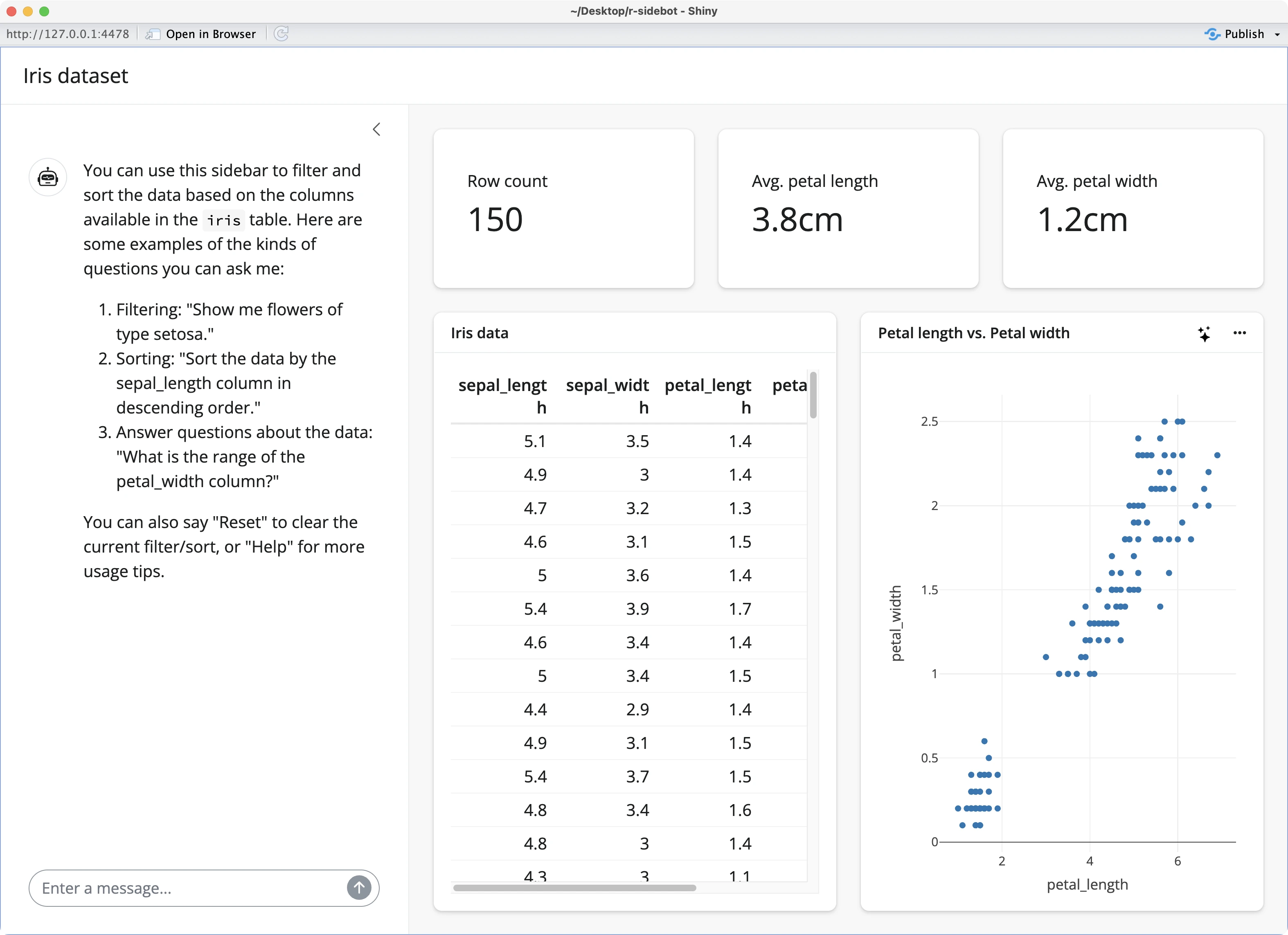
Image 18 - Customized Sidebot app (1)

But overall, the filtering operations applied through natural text work like a charm:
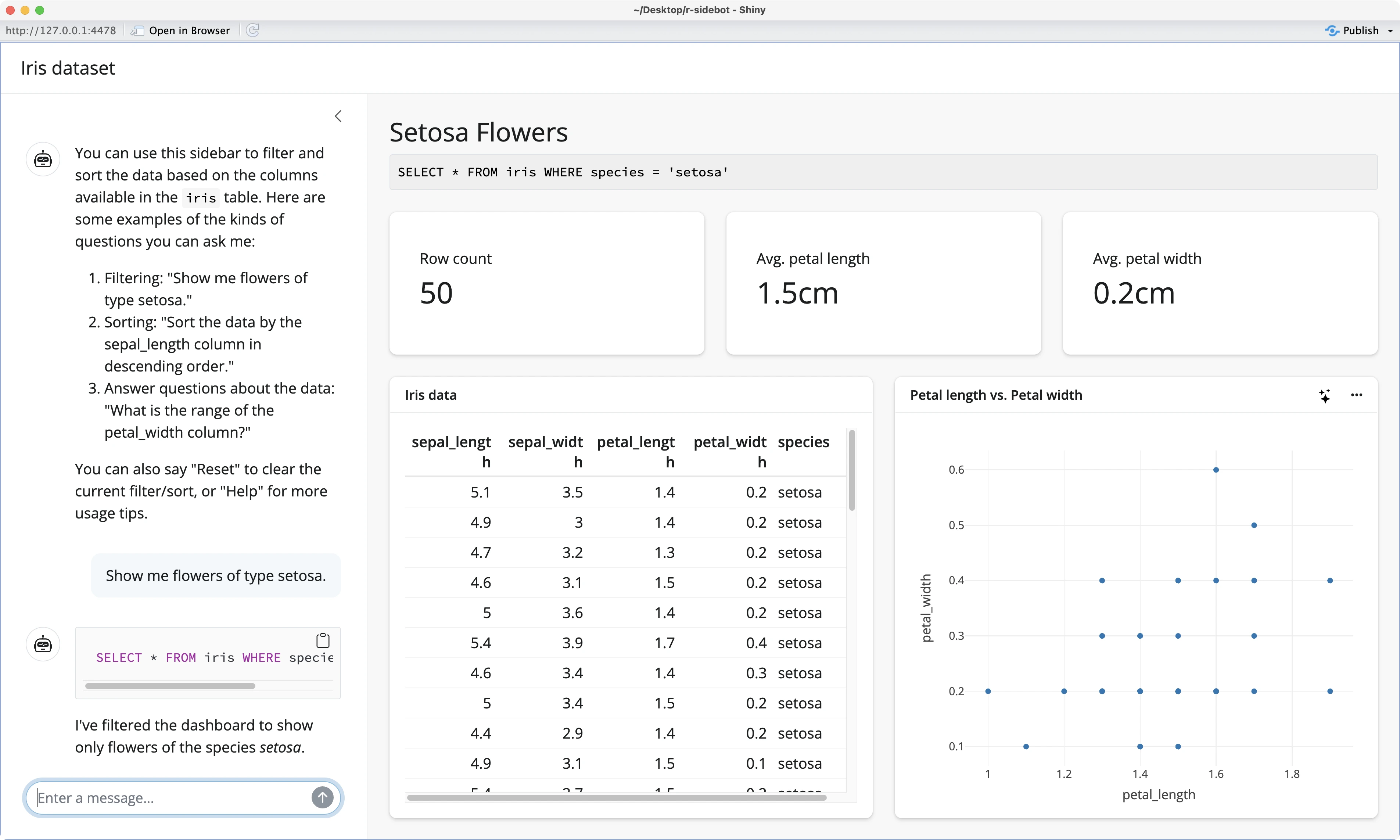
Image 19 - Customized Sidebot app (2)

And that’s it - you now know how to customize R Sidebot to work on your data!

Let’s make a brief recap next.

Summing up R Sidebot

Generative AI is here to stay.

Projects like R Sidebot perfectly demonstrate how much LLMs have matured over the years and how the amount of friction of using LLMs in your apps has decreased over time. Sure, the underlying packages such as elmer and shinychat are still experimental, but there’s no doubt in what the future holds.

At Applison, we’re proud to say that we’we successfully adopted LLMs in customer projects and in-house products. For example, we’be built Extractable, a tool that uses GPT to extract data from uploaded documents and transform it into standardized tables. We’ve also developed a Text2Graph application that allows you to transform your datasets into beautiful visualizations through natural text.

If your company can benefit from Large Language Models, feel free to reach out and tell us about your idea.

What are your thoughts on R Sidebot and LLMs as a replacement for traditional filters in apps and dashboards? Join our Slack community and let us know.

It’s one thing to write an R Shiny app, but deploying it comes with its own set of challenges. Read our 5 recommended deployment options for individuals and enterprises.

Have questions or insights?

Engage with experts, share ideas and take your data journey to the next level!

Is Your Software GxP Compliant?

Download a checklist designed for clinical managers in data departments to make sure that software meets requirements for FDA and EMA submissions.
Explore Possibilities

Share Your Data Goals with Us

From advanced analytics to platform development and pharma consulting, we craft solutions tailored to your needs.

Talk to our Experts
shiny