R Shiny and DuckDB: How to Speed Up Your Shiny Apps When Working With Large Datasets
If there’s one thing with a certain downward trend, it’s got to be people’s attention span. Even Google reports that pages with a load time of 5 seconds increase their probability of bounce by 90%! And that was in 2017!
As an R Shiny developer, you must do everything in your power to stop users leaving your app and increase engagement. One way to do it is to speed up data loading and processing time. Combining R Shiny and DuckDB is an excellent way to go.
In this article, you’ll learn what happens to R when you try to load over 200 million rows of data in your Shiny app, and what are the go-to ways to make it happen in seconds, not minutes.
Looking for an alternative way to process huge amounts of data? Try R dtplyr - A dplyr-like package with a data.table backend.
Table of Contents:
- DuckDB vs. Dplyr - How Much Faster is DuckDB On Real Data?
- Bringing DuckDB to R Shiny - How to Speed Up Slow Shiny Apps
- Summing up R Shiny and DuckDB
DuckDB vs. Dplyr - How Much Faster is DuckDB On Real Data?
We’ve already written about DuckDB on our blog, so we won’t repeat ourselves here. Today it’s all about hands-on experience.
The goal of this section is to test how much faster DuckDB is when compared to dplyr - a de facto standard analysis tool in R.
Dataset Configuration
If you want to follow along, you’ll need to download monthly Yellow Taxi trip data from 2019 to 2023 in Parquet format. You’ll end up with 60 individual data files, all taking around 3.3 GB of disk space:
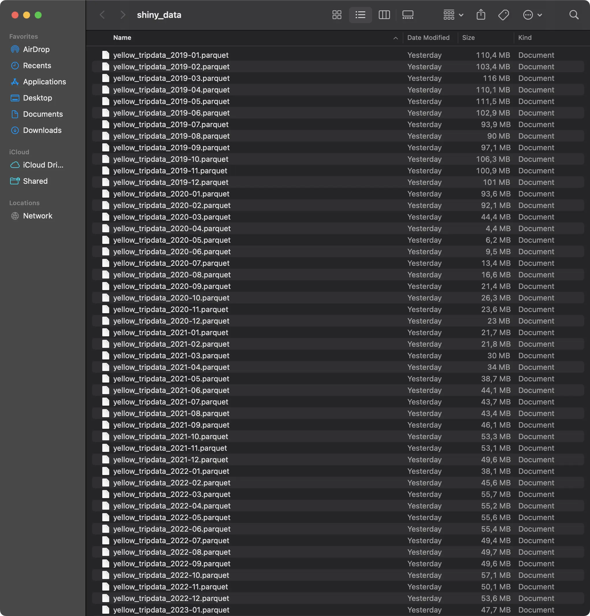
The Shiny application you’ll build shortly will load the data one year (12 Parquet files) at a time. For that reason, let’s also inspect how many rows of data you’ll be working with:

Short answer - a lot. Over 218 million in total, with 2019 alone having more than 84 million of recorded taxi rides. If even the idea of working with this amount of data in R Shiny makes your head spin, well, you’re not alone.
Required R Packages
You’ll need the following packages installed to follow along:
If any of these are not installed, simply run the `install.packages(“<package-name>”)` command from the R console to get you going.
Benchmark Function - Dplyr
Onto the fun stuff now!
The goal of this section is to write a function that reads one year’s worth of Parquet files from disk and performs some sort of aggregation. We’ll keep things simple and only calculate the basic statistics - number of rides, average duration, distance, price, tip amount, and total distance and price - all on a monthly basis.
If you know dplyr, the aggregation shouldn’t look foreign to you. What might look relatively new is the way you need to load the data. Put simply, the data is scattered between 12 Parquet files and you need a dynamic way to get the full file paths. Once you have that, you can use the `arrow::open_dataset()` function to turn the results into an Arrow table, and then into a data frame.
Here’s the full logic for our `get_dataset_for_year_dplyr()` function:
The function returns both the aggregated dataset and the time it took to read and parse the data. This second piece of information will be crucial for a comparison later.
Benchmark Function - DuckDB
Let’s now do the same but with DuckDB!
The `get_dataset_for_year_duckdb()` function accomplishes the same as the previous one, but by using DuckDB instead of dplyr. One clear benefit here is that you can use a Glob pattern to specify file locations instead of creating a list in a loop.
DuckDB allows you to write aggregations through dplyr-like functions or through SQL. We’ve opted for the latter, just to introduce some variety:
And now, let’s compare the two!
Dplyr vs. DuckDB Benchmark Results
Note: The actual runtimes you’ll get will depend on the hardware you’re running R on. For reference, we’re using a 16” M3 Pro Macbook Pro with 12 CPU cores and 36 GB of RAM. If you can feed more cores to the underlying DuckDB engine, you’ll likely be able to process the data even faster.
Running the `get_dataset_for_year_dplyr()` and `get_dataset_for_year_duckdb()` will return two values - the aggregated data and the runtime. Let’s take a peek into the data first:

It’s a nice, condensed, and informative overview of the millions of rows that went into the calculation.
As for the runtimes, the results are interesting:
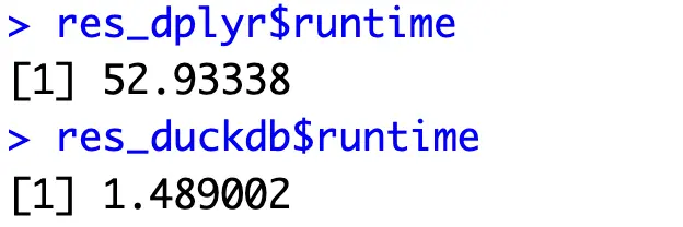
Remember the 5-second rule from the introduction? Imagine what would happen if the user had to wait almost a minute! To make things worse, you’ll probably host your Shiny app on a significantly less powerful server.
Nevertheless, DuckDB is a clear winner - being around 35x faster. Let’s now use it in R Shiny to see how that translates to application load speeds.
Bringing DuckDB to R Shiny - How to Speed Up Slow Shiny Apps
You’ll want to start by creating two files - `helpers.R` and `app.R`. In the prior, simply paste all the package imports and logic for our two data loading functions (Dplyr and DuckDB).
As for the latter, let’s get into it!
Shiny App Code
The application you’ll write now will be quite straightforward, as it will show one table and three charts. The user will be able to select a year from a dropdown menu, and the visuals will be rerendered once the data is loaded. You’ll also see the total loading time. It’s an unnecessary component for a production app, sure, but is here just to illustrate a point.
As for the external packages, you’ll want to make sure you’re comfortable with the following ones:
- DT: A package used to visualize table data in R and R Shiny. It has built-in search and pagination functionalities that will come in handy.
- Highcharter: Amazing package for producing interactive and animated visualizations for R and R Shiny.
The app is split into two parts - a sidebar that shows the title, filters, and the runtime in seconds, and a main panel that shows the visuals.
In the `server()` function, you’re free to change the data loading function (Dplyr or DuckDB) to see the performance differences between the two. The code snippet below uses the `get_dataset_for_year_duckdb()` function.
Anyway, here’s the full code snippet:
You can now run the app to see what it looks like:
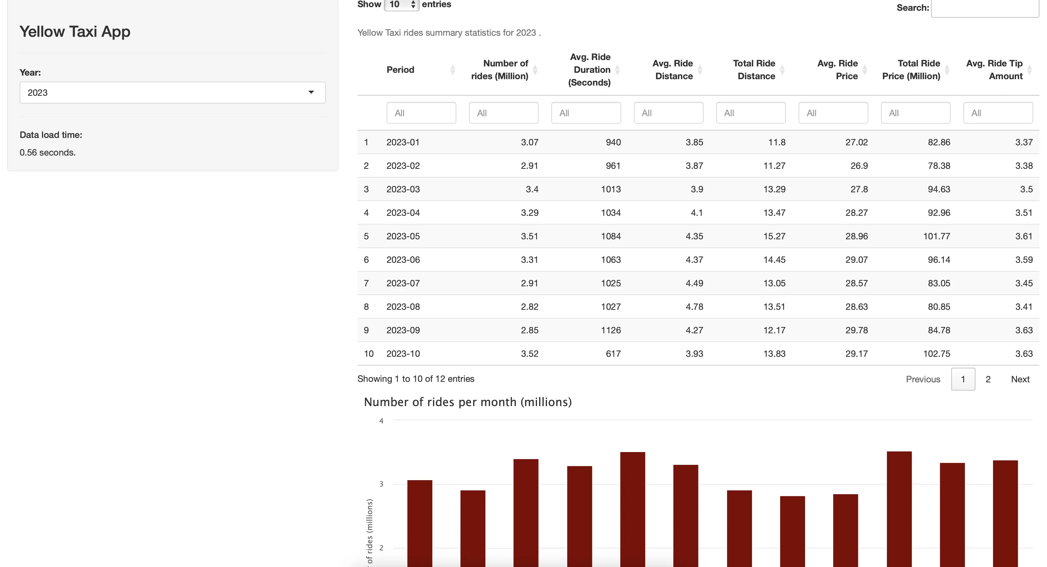
It seems like the data for 2023 loaded in around 0.5 seconds with DuckDB!
You can see the monthly statistics in a table form, or through three different charts:
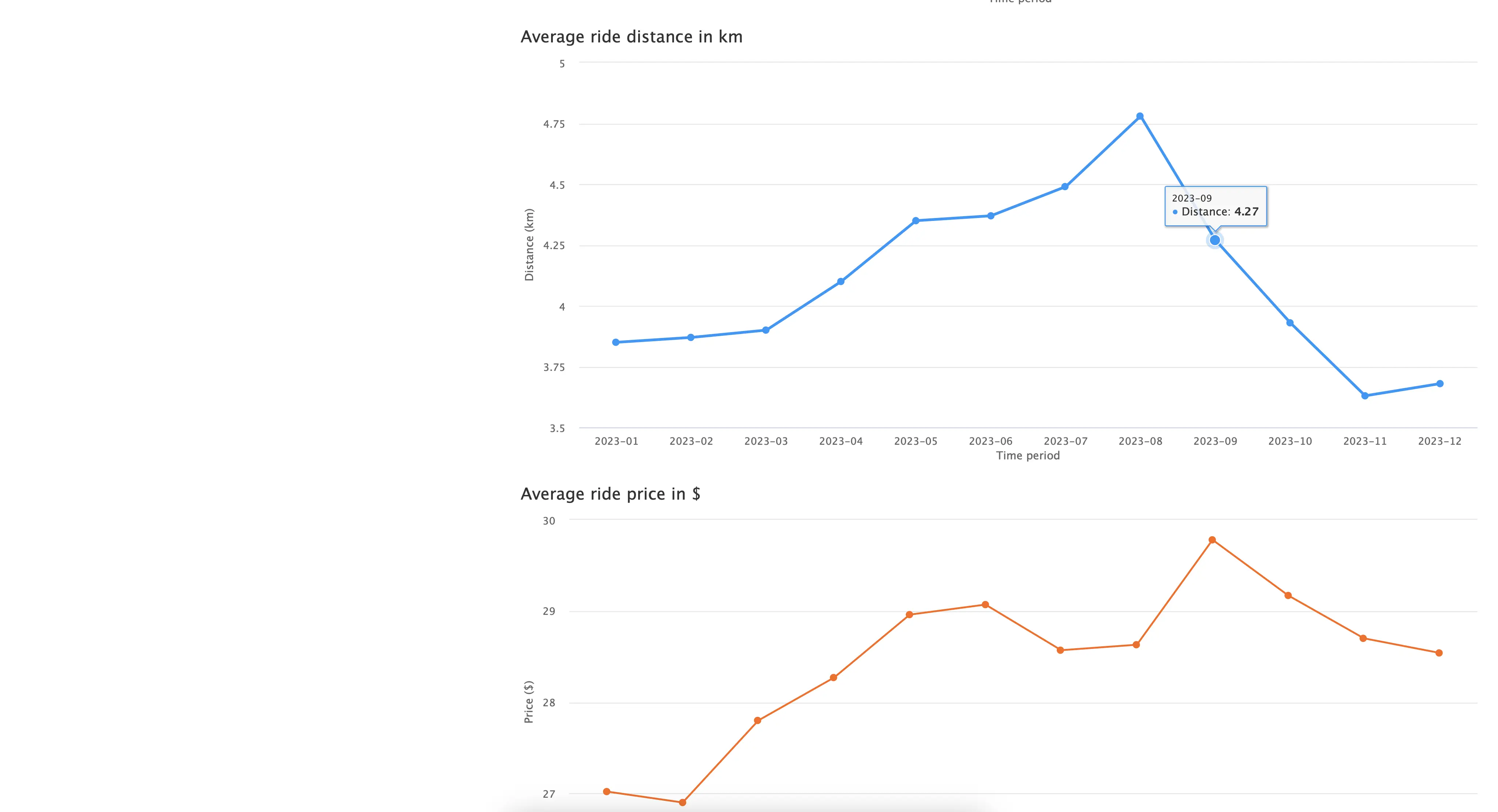
Overall, it’s a simple R Shiny application that could benefit from adding more content and tweaking the visuals, but we’ll leave that up to you.
Our task is to compare the runtime differences, so let’s start with dplyr.
Runtime Examination - Dplyr
Using the application version that runs the `get_dataset_for_year_dplyr()` function is a painful experience, to say the least. Cold starting the application took a painfully long 22 seconds:

But, things get worse as the data grows in size. For example, loading the 2019 data (84.5 million rows) took almost a minute:
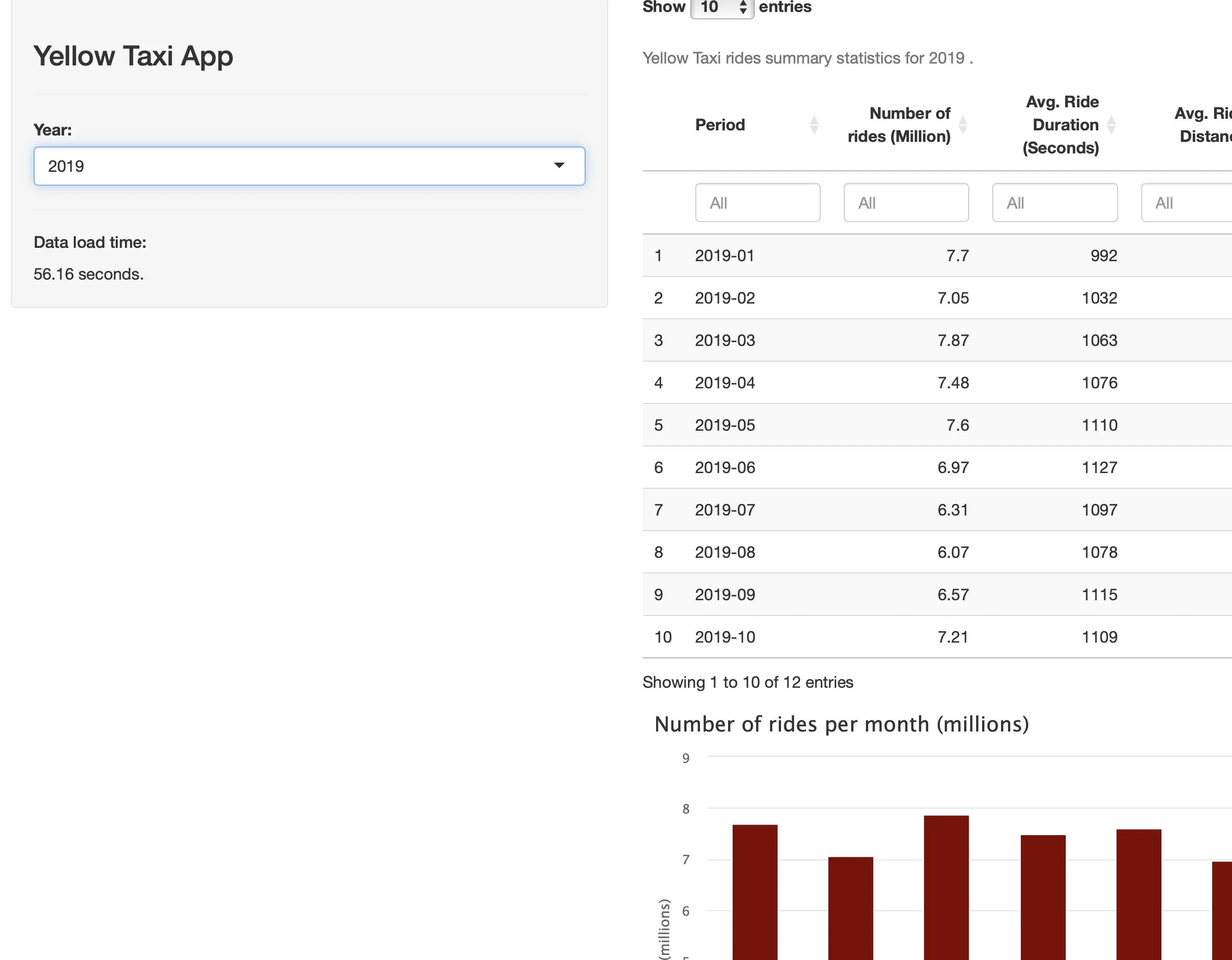
That’s a full minute that your user can’t interact with the application. Maybe the wait time is worth it, but we have our doubts.
Runtime Examination - DuckDB
Switching data processing backends from dplyr to DuckDB makes a world of difference. For example, loading the largest subset (2019) takes only 1.5 seconds:
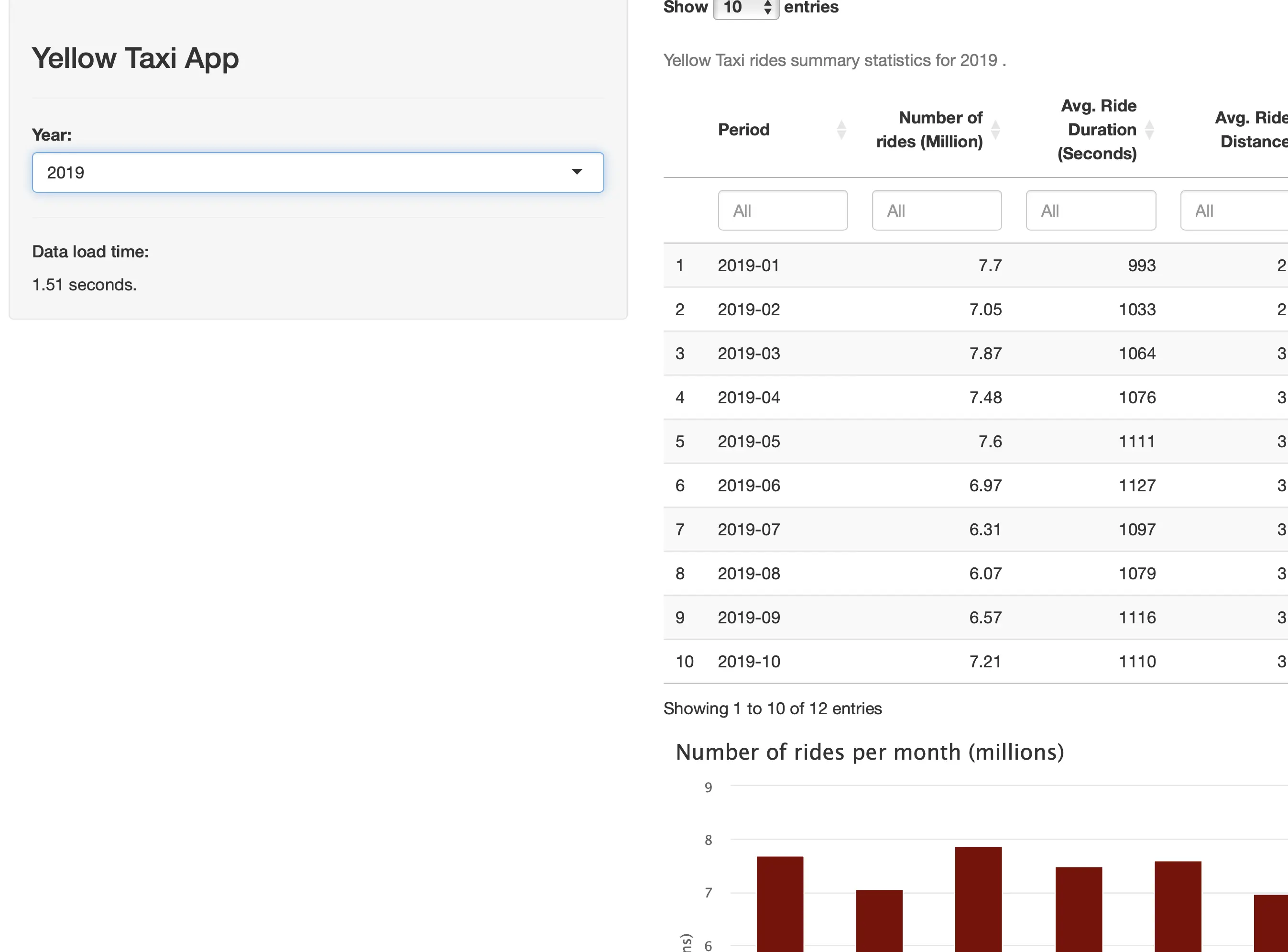
2022, which has just under 40 million rows is done loading and parsing in under 1 second:
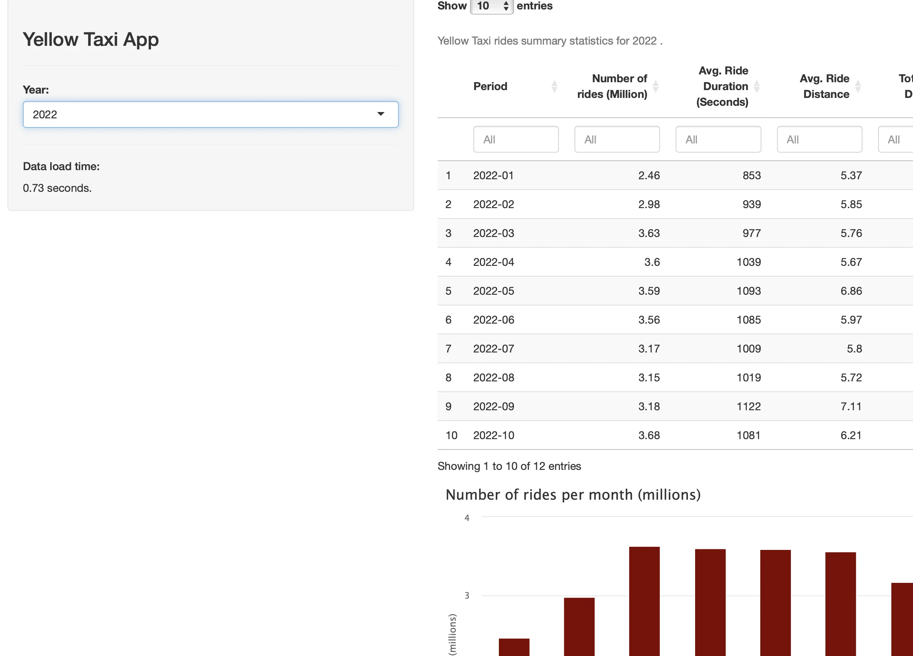
We don’t have much else to say, the numbers speak for themselves.
Runtime Comparison
To remove any chance of “luck” from our runtime comparison, we’ve run the data loading process in R Shiny 5 times for both Dplyr and DuckDB and for every year. Here are the average load time numbers:
Dplyr:
- 2019 - 56.54 seconds
- 2020 - 17.22 seconds
- 2021 - 19.03 seconds
- 2022 - 26.24 seconds
- 2023 - 25.69 seconds
DuckDB:
- 2019 - 1.51 seconds
- 2020 - 0.98 seconds
- 2021 - 0.66 seconds
- 2022 - 0.73 seconds
- 2023 - 0.61 seconds
In other words, Dplyr takes 0.61 to 0.7 seconds on average to read and parse 1 million rows of Parquet data, while DuckDB takes only 0.016 to 0.04 seconds for the same task.
Summing up R Shiny and DuckDB
To conclude, the technology you choose to read and process data for your Shiny app matters. It’s easy to point fingers at the web framework, but in reality, that’s almost never a bottleneck. You’ve seen just which sorts of performance improvements you can get by switching from Dplyr to DuckDB. It’s not even close!
Now, to get this level of performance from DuckDB you’ll need a powerful CPU with as many cores as you can get. On the other hand, R dplyr is single-threaded, so going for a 16-core CPU configuration in deployment scenarios doesn’t make much sense.
It’s a tradeoff between a fast-running application and a happy wallet. Optimize for what you need.
Your Shiny app works, but what’s next? It’s time to make it beautiful. Read our latest blog post to find out how.
