R dtplyr: How to Efficiently Process Huge Datasets with a data.table Backend

In a world where compute time is billed by the second, make every one of them count. There are zero valid reasons to utilize a quarter of your CPU and memory, but achieving complete resource utilization isn't always a straightforward task. That is if you don't know about R dtplyr.
One option is to use dplyr. It's simple to use and has intuitive syntax. But it's slow. The other option is to use data.table. It's lightning-fast but has a steep learning curve and syntax that's not too friendly to follow. The third - and your best option - is to combine the simplicity of dplyr with efficiency of data.table. And that's where R dtplyr chimes in!
Today you'll learn just how easy it is to switch from dplyr to dtplyr, and you'll see hands-on the performance differences between the two. Let's dig in!
Looking for an alternative R data processing framework? Our detailed benchmark and comparison has you covered.
Table of contents:
- What is R dtplyr And Why Should You Care?
- How to Install R Dtplyr and Data Table the Right Way
- R dplyr vs. dtplyr - Which R Data Processing Package is Faster?
- Summing up R dtplyr
What is R dtplyr And Why Should You Care?
R dtplyr is an R package that works almost identically to dplyr on the frontend but differs in the backend in some key ways. You can use both packages to efficiently manipulate and aggregate data using friendly syntax - no difference there - but what sets them apart is dtplyr's ability to work with larger-than-memory datasets.
One of the main pain points users have with plain dplyr is its slow performance on large datasets. This is frustrating, especially for the reason we mentioned in the introduction (time is money). If you need data processing done quickly, dplyr isn't the option you should opt for.
A reasonable alternative might be the data.table package, as it can work with huge datasets rather efficiently. The problem is, it comes with difficult-to-master syntax, and learning it is both time-consuming and frustrating since the syntax is way harder to understand when compared to dplyr.
The solution? What if you could use the processing power of data.table while writing dplyr-like syntax? That's exactly what R dtplyr does.
The goal is to let dtplyr worry about translating dplyr code to data.table code, and for you to have a good time in the process. For the translation reason, dtplyr will always be a tad slower than data.table, but it's a price worth paying.
As a developer, all you have to remember is to convert data.frames to tibble objects before using dtplyr and to call lazy_dt() after your first pipe sign. That's it - everything else it the same as with dplyr.
When it comes to using R dtplyr, the installation itself isn't the most intuitive on macOS, but the package can be installed without hiccups on other operating systems. We'll describe the installation process next.
How to Install R Dtplyr and Data Table the Right Way
On Mac devices, even with Apple Silicon, a lot of users are reporting various warning messages telling them data.table is running in a single-threaded mode. That's usually not what you want, as it will significantly prolong the overall computation time.
Truth be told, if your dplyr calculations are fast (seconds), it doesn't make sense to use dtplyr in a multi-threaded mode just because the additional thread overhead will eat into your total runtime. You'll see how and why in the following section.
Folks over at Stack Overflow have come up with a solution that fixes single-threaded issues for Mac users. We'll go over it now.
Traditionally, this is how you would install R packages (this will work on most operating systems):
install.packages(c("data.table", "dtplyr"))
You can now load them and see if there are any warning messages:
library(data.table)

It looks like there are, and data.table is running in a single-threaded mode. Let's fix it!
To start, you'll need to uninstall any previous installation of data.table from your system. You can do that by running the following command in the R console:
remove.packages("data.table")
From there, install the following Mac packages via Homebrew:
brew install libomp
brew install pkg-config
Now create a Makevars file:
mkdir ~/.R
nano ~/.R/Makevars
And paste the following inside the file. Save it once you're done and you'll be good to go:
LDFLAGS += -L/opt/homebrew/opt/libomp/lib -lomp
CPPFLAGS += -I/opt/homebrew/opt/libomp/include -Xclang -fopenmp
You can now install data.table from source within the R shell:
install.packages("data.table", type = "source")
If you were to load the data.table package now, you wouldn't get any of the single-threaded error or warning messages:
library(data.table)

You now have data.table installed properly on your device, so we can continue with the benchmarks.
R dplyr vs. dtplyr - Which R Data Processing Package is Faster?
R dtplyr works best on larger datasets, so we'll show you how to create one with 10M rows next!
Dataset Creation
You'll need the following R packages to follow along. Use the install.packages("package-name") command to install any if missing, and make sure to follow our custom data.table installation guide if you're using macOS:
library(dtplyr)
library(ggplot2)
library(data.table)
library(stringi)
library(cleaner)
library(lubridate)
Onto the dataset creation. The data.frame will have 10 million rows with a mixture of textual, numeric, and datetime types. All values are random, have no association with the real world, and are here only to demonstrate a point:
n <- 10000000

data <- data.frame(
  id = 1:n,
  dt = rdate(n, min = "2000-01-01", max = "2024-01-01"),
  str = stri_rand_strings(n, 4),
  num1 = rnorm(n),
  num2 = rnorm(n, mean = 10, sd = 2),
  num3 = rnorm(n, mean = 100, sd = 10)
)

head(data)

We now have the dataset, so next we can start with the benchmarks.
R dplyr Benchmarks
Let's begin with the package you're already familiar with - dplyr. It will serve as a baseline that we'll want to outperform.
All test durations will be measured using Sys.time() and will be wrapped in a custom R function.
Let's briefly explain each of the functions:
dplyr_bench_1()- Returns the count of rows based on a filtered-down version of the dataset,dplyr_bench_2()- Groups the data by thestrcolumn, calculates summary statistics, and reorders the dataset.dplyr_bench_3()- Groups the data by year (extracted from a derived column), calculates summary statistics and reorders the dataset.
All benchmark functions are rather simple, but it'll be interesting to see how much time they'll require due to a somewhat large number of rows:
dplyr_bench_1 <- function(dataset) {
  start_time <- Sys.time()

  res <- dataset %>%
    filter(num3 > 130) %>%
    summarise(count = n()) %>%
    as_tibble()

  end_time <- Sys.time()
  duration <- end_time - start_time

  print(duration)

  return(res)
}

dplyr_bench_2 <- function(dataset) {
  start_time <- Sys.time()

  res <- dataset %>%
    group_by(str) %>%
    summarise(
      n_rows = n(),
      avg_num1 = mean(num1),
      avg_num2 = mean(num2),
      avg_num3 = mean(num3)
    ) %>%
    arrange(desc(n_rows)) %>%
    as_tibble()

  end_time <- Sys.time()
  duration <- end_time - start_time

  print(duration)

  return(res)
}

dplyr_bench_3 <- function(dataset) {
  start_time <- Sys.time()

  res <- data %>%
    mutate(year = year(dt)) %>%
    group_by(year) %>%
    summarise(
      n_rows = n(),
      avg_num1 = mean(num1),
      avg_num2 = mean(num2),
      avg_num3 = mean(num3)
    ) %>%
    arrange(desc(n_rows)) %>%
    as_tibble()

  end_time <- Sys.time()
  duration <- end_time - start_time

  print(duration)

  return(res)
}
Once you have these functions in your R environment, run the following snippet line by line:
dplyr_res_1 <- dplyr_bench_1(data)
dplyr_res_2 <- dplyr_bench_2(data)
dplyr_res_3 <- dplyr_bench_3(data)
These are the results we got:

The first and the third functions were fast to run, but the second took almost 3 minutes! Let's see if dtplyr can offer any performance benefits.
R dtplyr Benchmarks
As mentioned before, you need to convert your data.frame to tibble before applying dtplyr functions to your data:
dtplyr_data <- as_tibble(data)
The benchmark functions are almost exactly the same, with one exception - each of them calls lazy_dt() before doing anything else:
dtplyr_bench_1 <- function(dataset) {
  start_time <- Sys.time()

  res <- dataset %>%
    lazy_dt() %>%
    filter(num3 > 130) %>%
    summarise(count = n()) %>%
    as_tibble()

  end_time <- Sys.time()
  duration <- end_time - start_time

  print(duration)

  return(res)
}

dtplyr_bench_2 <- function(dataset) {
  start_time <- Sys.time()

  res <- dataset %>%
    lazy_dt() %>%
    group_by(str) %>%
    summarise(
      n_rows = n(),
      avg_num1 = mean(num1),
      avg_num2 = mean(num2),
      avg_num3 = mean(num3)
    ) %>%
    arrange(desc(n_rows)) %>%
    as_tibble()

  end_time <- Sys.time()
  duration <- end_time - start_time

  print(duration)

  return(res)
}

dtplyr_bench_3 <- function(dataset) {
  start_time <- Sys.time()

  res <- dataset %>%
    lazy_dt() %>%
    mutate(year = year(dt)) %>%
    group_by(year) %>%
    summarise(
      n_rows = n(),
      avg_num1 = mean(num1),
      avg_num2 = mean(num2),
      avg_num3 = mean(num3)
    ) %>%
    arrange(desc(n_rows)) %>%
    as_tibble()

  end_time <- Sys.time()
  duration <- end_time - start_time

  print(duration)

  return(res)
}
Like before, make sure to run this code snippet line by line:
dtplyr_res_1 <- dtplyr_bench_1(dtplyr_data)
dtplyr_res_2 <- dtplyr_bench_2(dtplyr_data)
dtplyr_res_3 <- dtplyr_bench_3(dtplyr_data)

The first and the third functions took longer to run, but the second one was over 20 times faster! That's some serious compute time reduction, and we'll explain the reasons behind it in the following section.
Benchmark Result Comparison
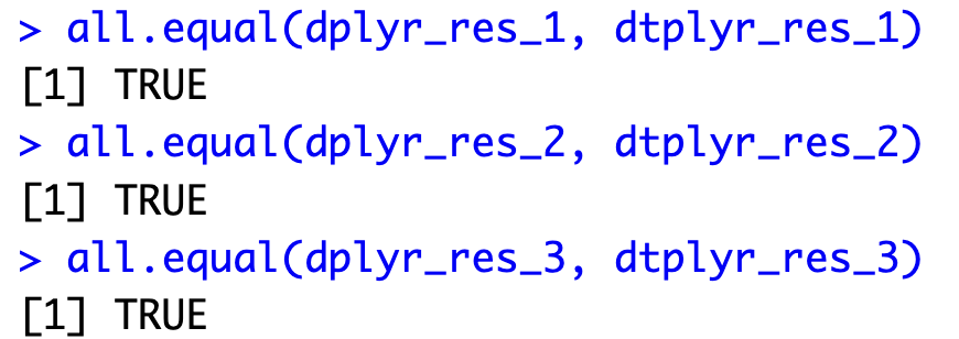
Before interpreting results, it's worth to take a minute to compare the returned values. After all, our benchmark is only meaningful if the code outputs are identical.
You can use the all.equal() function to compare two tibbles:
all.equal(dplyr_res_1, dtplyr_res_1)
all.equal(dplyr_res_2, dtplyr_res_2)
all.equal(dplyr_res_3, dtplyr_res_3)

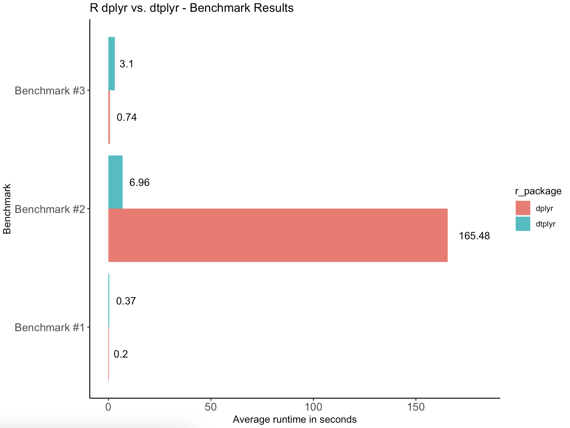
It looks like the outputs are identical, so let's go over the results one more time - visually now:
ggplot(res_df, aes(x = benchmark, y = times, fill = r_package)) +
  geom_col(position = position_dodge()) +
  coord_flip() +
  geom_text(aes(label = times), position = position_dodge(0.9), hjust = -0.35, size = 4, color = "#000000") +
  scale_y_continuous(limits = c(0, max(res_df$times) * 1.1)) +
  labs(
    title = "R dplyr vs. dtplyr - Benchmark Results",
    x = "Benchmark",
    y = "Average runtime in seconds"
  ) +
  theme_classic() +
  theme(
    axis.text.x = element_text(size = 12),
    axis.text.y = element_text(size = 12)
  )

Wondering how we made this chart? Follow our guide to stunning bar charts with ggplot2.
In a nutshell:
- R dtplyr took longer to execute short-running tasks. This is somewhat reasonable because we're running
data.tablecalculations on 6 threads in our case, and setting them up and managing them takes time. There'll always be some overhead when compared to single-threaded executions. - On a longer-running calculation, R dtplyr was consistently over 20 times faster than vanilla dplyr. This is where multi-threaded execution and optimized backend really stand out.
- In total, dplyr took 166 seconds to finish all three tests, while dtplyr took only 10 seconds. It's a significant improvement to say at least.
Long-running calculations make dtplyr stand out and drastically reduce the overall compute time. That's why it's an essential package to know when your compute time is billed by the second.
Summing up R dtplyr
To conclude, you should absolutely know about R dtplyr if you're working with large datasets. There's no reason not to use it since you're probably already using vanilla dplyr to analyze data. This package keeps the developer-friendly syntax and ease of use, all while bringing the speed of data.table into the mix.
R dtplyr usually runs on multiple threads, so you'll generally want to use it on tasks that run longer than a couple of seconds. There's no one stopping you from using it all the time - but you'll have to pay the price for initializing and managing multiple threads, so keep that in mind.
Ever wondered how Python's Pandas compares to dplyr? We have the answer.

.png)


.png)